Creating summaries of trip rates

To calculate trip rates we first need to prepare the data. We can do this using hts_prep_triprate

library(travelSurveyTools)
library(ggplot2)

## Warning: package 'ggplot2' was built under R version 4.3.2

data("test_data")
data("variable_list")
data("value_labels")

prepped_triprates_list = hts_prep_triprate(
  variables_dt = variable_list,
  trip_name = "trip",
  day_name = "day",
  hts_data = test_data
)

After preparing the data we can create a summary using hts_summary.

hts_summary(
  prepped_dt = prepped_triprates_list$num,
  summarize_var = "num_trips_wtd",
  summarize_vartype = "numeric"
)

## $n_ls
## $n_ls$unwtd
## $n_ls$unwtd$`Count of unique day_id`
## [1] 4125
## 
## $n_ls$unwtd$`Count of unique person_id`
## [1] 1760
## 
## $n_ls$unwtd$`Count of unique hh_id`
## [1] 825
## 
## 
## $n_ls$wtd
## NULL
## 
## 
## $summary
## $summary$unwtd
##    count min      max    mean   median
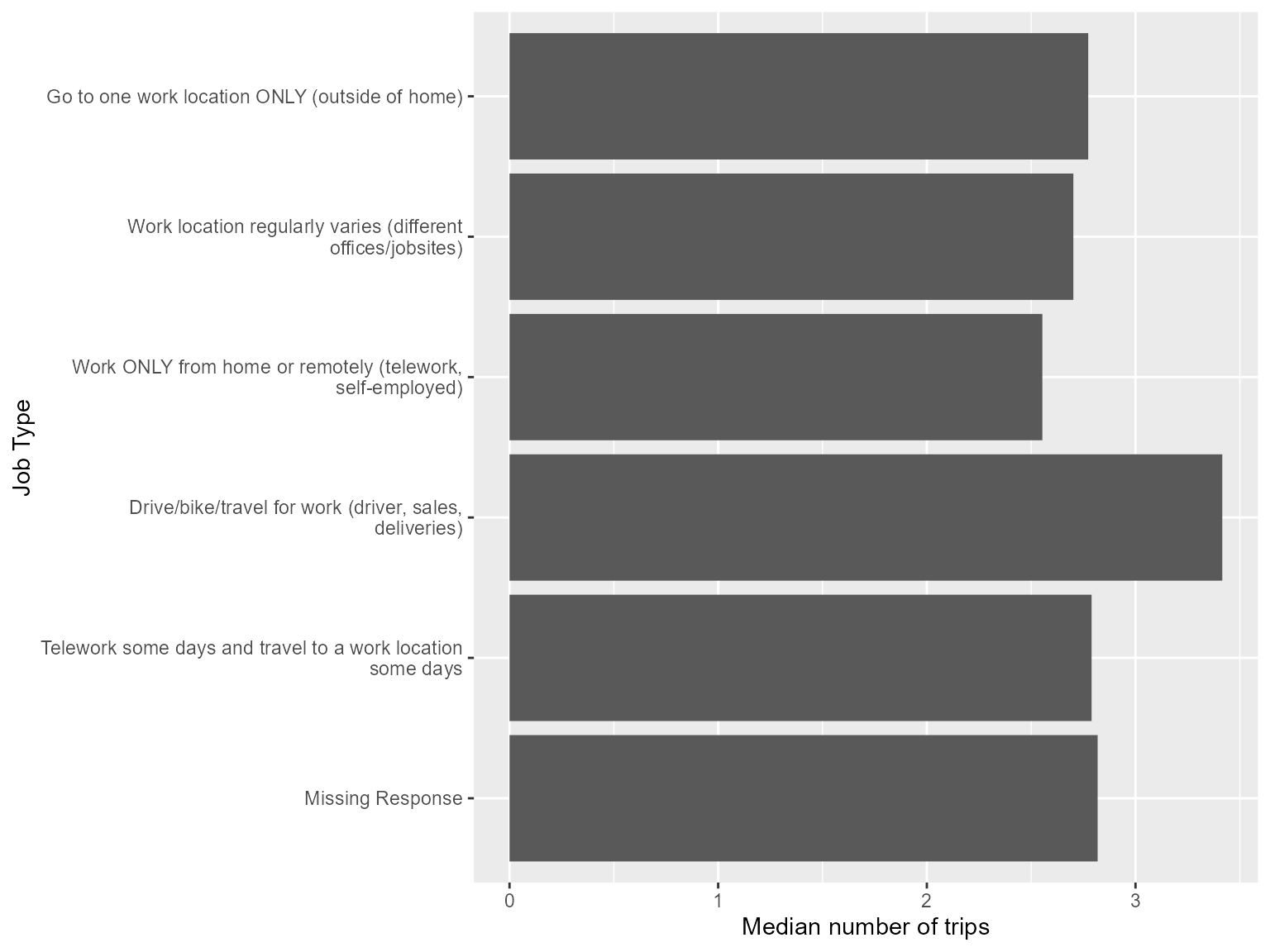
## 1:  4125   0 391.8182 9.69461 3.719258

We can also summarize trip rates by one or more variables.

job_type_triprate_list = hts_prep_triprate(
  variables_dt = variable_list,
  summarize_by = "job_type",
  trip_name = "trip",
  day_name = "day",
  hts_data = test_data
)

num_trips_job_type = hts_summary(
  prepped_dt = job_type_triprate_list$num,
  summarize_by = "job_type",
  summarize_var = "num_trips_wtd",
  summarize_vartype = "numeric",
  wtname = "day_weight",
  weighted = TRUE
)$summary$wtd



# Label job_type
num_trips_job_type_labeled = factorize_df(
  num_trips_job_type,
  value_labels,
  value_label_colname = "label"
)


# Create a plot
ggplot(
  num_trips_job_type_labeled,
  aes(x = median, y = job_type)
) +
  geom_bar(stat = "identity") +
  scale_y_discrete(
    labels = function(x) stringr::str_wrap(x, width = 50),
    limits = rev
  ) +
  labs(
    x = "Median number of trips",
    y = "Job Type"
  )

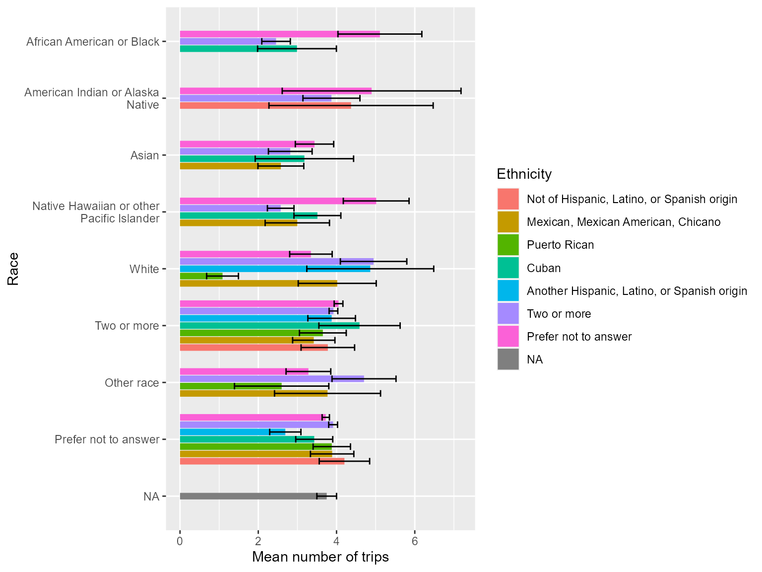
race_ethnicity_triprate_list = hts_prep_triprate(
  variables_dt = variable_list,
  summarize_by = c("race", "ethnicity"),
  trip_name = "trip",
  day_name = "day",
  hts_data = test_data
)

num_trips_race_ethnicity = hts_summary(
  prepped_dt = race_ethnicity_triprate_list$num,
  summarize_by = c("race", "ethnicity"),
  summarize_var = "num_trips_wtd",
  summarize_vartype = "numeric",
  wtname = "day_weight",
  weighted = TRUE,
  se = TRUE
)$summary$wtd

# label data
num_trips_race_ethnicity_labeled = factorize_df(
  num_trips_race_ethnicity,
  value_labels,
  value_label_colname = "label"
)

# Create a plot
ggplot(
  num_trips_race_ethnicity_labeled,
  aes(x = mean, y = race, fill = ethnicity)
) +
  scale_y_discrete(
    labels = function(x) stringr::str_wrap(x, width = 30),
    limits = rev
  ) +
  geom_bar(stat = "identity", position = position_dodge2(preserve = "single", width = 0)) +
  geom_errorbar(
    aes(
      xmin = (mean - mean_se),
      xmax = (mean + mean_se)
    ),
    position = position_dodge2(preserve = "single", width = 0)
  ) +
  labs(
    x = "Mean number of trips",
    y = "Race",
    fill = "Ethnicity"
  )