# Load hts.weighting Package
devtools::load_all()

# Load Settings; Pass python_env Explicitly for Quarto
settings = get_settings(reload_settings = TRUE,
                        print = FALSE)

# Set Pathways for Reference
code_root = get("code_root", settings)
work_dir = get('working_dir', settings)
inputs_dir = get('inputs_dir', settings)
outputs_dir = get('outputs_dir', settings)
report_dir = get('report_dir', settings)
popsim_initial_label = get("popsim_initial_label", settings)
popsim_daypat_label = get("popsim_daypat_label", settings)8 Round 1 Weighting: Demographic Calibration
8.1 Overview
The goal of this chapter is to produce weights that achieve a balance between these two (sometimes competing) objectives:
- Fit the survey data as closely as possible to the Census target data.
- Minimize variance in the weights to avoid overly high, low, or skewed weights.
To achieve this goal, weights are fit iteratively and this step will likely be run several times before achieving the desired fit.
What You’ll Do
- Calculate base weights for each household based on their probability of inclusion.
- Configure and prepare the data and settings for PopulationSim.
- Run PopulationSim to generate diagnostic outputs and final Round 1 weights.
- Review weight variability, error, and fit to targets by zone and region.
Multiple rounds of weighting are common in survey statistics. In this case, the first round of weighting serves two purposes:
- Calibrate the weighting configuration: this round is used to adjust the targets supplied to, and constraints placed upon, the weighting algorithm.
- Generate weights for bias adjustment models: Weights generated in Round 1 are used to create weighted day-pattern bias models; without them, models would be unweighted and subject to sampling bias, and less reflective of the population overall.
This section begins by estimating the base weight for each household based on their probability of being included in the final sample. Then, base weights are input into PopulationSim and adjusted for non-response bias across geographies and demographics (Round 1 weighting). This chapter concludes with a series of tables and figures to review the output of Round 1 weighting and determine if adjustments are needed.
What is PopulationSim?
PopulationSim is an open-source software package originally designed for population synthesis in travel demand modeling, but it also functions as a survey weighting engine when integerization is disabled. Its key advantage for household travel surveys is that it can operate on data with a nested household-person structure and can enforce consistency across multiple geographic levels. PopulationSim’s infrastructure also allows integration across multiple geographic levels, such as household weighting zones (i.e., PUMAs) and larger weighting zone groups.
8.2 Base Weight Estimation
Base weights represent each respondent’s probability of inclusion in the final sample and serve as the foundation for all further weighting steps. These probabilities combine both the probability of selection (how likely a household is to be invited to participate) and the probability of response (how likely a household is to complete the survey).
The probability of inclusion for each sample segment is calculated with the following formulas:
Formula inputs
- m: number of mailed invites in the sample segment
- H: total number of households in the sample segment (estimated from 5-year ACS data)
- R: number of responses (complete households) in the sample segment BW: base weight for a given sample segment
\[ P_{\text{selection}} = \frac{m}{H} \]
\[ P_{\text{response}} = \frac{R}{m} \]
Thus, the base weight for each sample segment is:
\[ P_{\text{inclusion}} = P_{\text{selection}} \times P_{\text{response}} = \frac{m}{H} \times \frac{R}{m} = \frac{R}{H} \]
\[ BW_{\text{segment}} = \frac{1}{P_{\text{inclusion}}} = \frac{H_{\text{segment}}}{R_{\text{segment}}} \]
For example, if segment A contains 100 households and the survey collected responses from 5 households, each household in that segment would have a base weight of 20 (100 / 5 = 20).
Load Settings and Define File Paths
Load Data
Load in the sample plan reference count data, the target estimates by weighting zones, and the seed (survey) data for calculating base weights.
# Load Unadjusted and Adjusted Sample Plan Tables.
sample_plan_adj = readRDS(file.path(get("working_dir", settings), "sample_plan_adj.rds"))
sample_plan = readRDS(file.path(get("working_dir", settings), "sample_plan_unadj.rds"))

# Load Target Estimate Data
target_czone = readRDS(get("target_czone_path", settings))

# Load Seed (Survey) Data and Day Table.
seed = readRDS(get("seed_path", settings))
day = fetch_hts_table("day", settings)
Calculate Base Weights
Base weights for each household in the seed (survey) dataset are calculated by dividing the (adjusted or unadjusted) reference count by the number of responding households in each sample segment. This produces weighted counts for each segment that reflect both the sample design and population targets.
# Load Unadjusted and Adjusted Sample Plan Tables.
sample_plan_adj = readRDS(file.path(get("working_dir", settings), "sample_plan_adj.rds"))
sample_plan = readRDS(file.path(get("working_dir", settings), "sample_plan_unadj.rds"))

# Load Seed (Survey) Data and Day Table.
seed = readRDS(get("seed_path", settings))
day = fetch_hts_table("day", settings)

# Calculate Base Weights Using the Unadjusted Sample Plan
seed_wtd_unadj = calc_initial_weights(sample_plan, seed, target_czone, settings, blend = TRUE)

# Record Checksum for Base Weights (Adjusted).
seed_wtd = calc_initial_weights(sample_plan_adj, seed, target_czone, settings, blend = TRUE)
Check That Base Weights Match Target Counts
This quality check verifies that the sum of base weights in the seed data closely matches the expected counts from weighting zone targets, within a defined threshold. This step is critical for identifying mismatches between the sample and population.
Checking base weights before adjusting weighting zone targets to sample segments…
Checking base weights (5-year ACS) against PUMS targets (1-year ACS)...
Day group: avg_weekday
    PER: 3373869 (5-year), 4243682 (1-year), -20.5%
    HH: 1673496 (5-year), 1745353 (1-year), -4.12%
Reference counts are within  Inf%  of the expected values.
Checking base weights after adjusting weighting zone targets to sample segments…
Checking base weights (5-year ACS) against PUMS targets (1-year ACS)...
Day group: avg_weekday
    PER: 3516845 (5-year), 4243682 (1-year), -17.13%
    HH: 1745353 (5-year), 1745353 (1-year), 0%
Reference counts are within  <0.1%  of the expected values.
A large difference in the person count can be expected as  a result of response bias from large-households in our survey.
Save Base Weight Output Files
# Save Base Weights
saveRDS(seed_wtd, get('seed_wtd_path', settings))
Table: Base weights by Sample Segment
Sample Segment | Sampled Households | Target | Base Weight |
|---|---|---|---|
King County-General | 456 | 456,148 | 1,000.32 |
King County-Hard-to-survey | 250 | 250,307 | 1,001.23 |
King County-Rural | 76 | 67,180 | 883.94 |
King County-Walk/Bike/Transit | 389 | 186,975 | 480.66 |
Kitsap County-General | 81 | 56,542 | 698.05 |
Kitsap County-Hard-to-survey | 14 | 11,700 | 835.74 |
Kitsap County-Rural | 43 | 43,394 | 1,009.17 |
Pierce County, Incorporated-General | 120 | 139,196 | 1,159.97 |
Pierce County, Incorporated-Hard-to-survey | 48 | 62,885 | 1,310.10 |
Pierce County, Rural (All) | 483 | 68,477 | 141.77 |
Pierce County, Unincorporated-General | 498 | 67,241 | 135.02 |
Pierce County, Unincorporated-Hard-to-survey | 116 | 14,359 | 123.78 |
Snohomish County-General | 231 | 210,373 | 910.71 |
Snohomish County-Hard-to-survey | 55 | 52,861 | 961.10 |
Snohomish County-Rural | 50 | 57,715 | 1,154.31 |
Total | 2,910 | 1,745,353 |
8.3 Round 1 Weighting
Overview
This step uses PopulationSim to adjust base weights for non-response and sampling error across geographies and demographics.
Key Concept: Non-response bias
Non-response bias refers to biases in the unweighted data that occur because different types of people respond to surveys at different rates.
What Does PopulationSim Do During Weighting?
PopulationSim applies the constrained entropy-maximization (EM) algorithm, a method widely used across survey weighting applications (including the U.S. Census Bureau’s Entropy-Based Weighting system). The goal is to adjust a set of starting weights (the seed) so that weighted survey estimates match a set of external targets. PopulationSim is run to adjust the household-level weights after calculating the base weights (Round 1), and again after adjusting the household-level weights for day patterns (Round 2). This is to ensure that weighted estimates using the data match selected characteristics of the population (i.e., “targets”) that may be over- or under-represented in the data due to non-response or sampling error.
To demonstrate how PopulationSim generates weights, consider the example below. If there were only a single weighting zone group with only a single target (e.g., household size), this step would simply adjust the base weights such that the distribution of the Round 1 weights matches the distribution of selected target variables.
In this example, assume each of 5 households has a base weight of 20.0 and a distribution of household sizes in the survey sample (unweighted) is as follows:
40% of households have 1 member
40% of households have 2 members
20% of households have 3 members
The distribution of household sizes in the target population (Census) is as follows:
20% of households have 1 member
40% of households have 2 members
40% of households have 3 members
The base weights for households with a size of 1 would be scaled down to match the targets, and base weights for households with a size of 3 would be scaled up to match the targets. The table below shows what the base weights would be after Round 1.
| Household size | Base weight | Round 1 weight | |
|---|---|---|---|
| Household 1 | 1 | 20.0 | 10.0 |
| Household 2 | 2 | 20.0 | 20.0 |
| Household 3 | 1 | 20.0 | 10.0 |
| Household 4 | 2 | 20.0 | 20.0 |
| Household 5 | 3 | 20.0 | 40.0 |
Prepare Data for PopulationSim
PopulationSim requires a set of input files for the weighting process:
- settings.yaml: Main configuration file containing all parameters for the weighting run.
- control.csv: Lists the control fields (target variables) and their assigned importance.
- seed.csv: Contains the processed survey data (seed data) to be weighted.
- control_totals_
.csv : Provides control totals for each geography (i.e., weighting zone or zone group, region) used as targets. - geo_crosswalk.csv: Maps geographies between seed data and targets to ensure correct aggregation.
The data files ensure that both the survey sample and target estimates are available at the correct geographic level for weighting.
Load Survey Seed and Target Data
The first step in Round 1 weighting is to assemble all necessary input data for PopulationSim. This includes:
- The seed data, which is the survey dataset with base weights already applied to each household record.
- Target estimates for each weighting zone (client zone or PUMA), which represent population and household control totals derived from ACS and PUMS data.
- Regional targets, providing aggregate population and household totals for the entire study region.
- Tabulated ACS PUMS data, which contains detailed breakdowns of household and person-level characteristics, ensuring demographic targets match the survey year.
- Geographic crosswalks, mapping survey records to weighting zones and zone groups, ensuring proper aggregation and alignment for weighting.
# Load Seed (Survey) Data with Base Weights
seed = readRDS(file.path(work_dir, 'survey_initial_wts.rds'))

# Load Target Estimates for Weighting Zones and Region
czone_targets = readRDS(get("target_czone_path", settings))
region_target = readRDS(get("target_region_path", settings))

# Load Tabulated ACS PUMS Data for Control Totals
pums_tabbed = readRDS(file.path(work_dir, "pums_tabbed.rds"))

# Load Crosswalk Mapping PUMAs to Client Zones
puma_client_zone_xwalk = readRDS(file.path(work_dir, "puma_czone_xwalk.rds"))
Create the PopulationSim Geographic Crosswalk
PopulationSim uses geographic crosswalks to connect the survey data to the geographic regions used for weighting. This step builds the crosswalk table:
- Weighting zone: The fundamental geographic unit used for weighting, often a PUMA or client zone, based on the ACS data or custom client needs.
- Weighting zone group: An aggregation of zones, created to ensure sufficient sample size and reliable target estimates. This is especially useful when zones (like small PUMAs) are grouped for stability.
PopulationSim allows aggregation of target estimates from individual weighting zones to zone groups as specified in the project settings. These crosswalks are saved for use in the weighting run.
# Create the PopulationSim Crosswalk Table, Used for Mapping Zones in Weighting.----------------------------------------
zone_group_crosswalk = prepare_zone_groups(
    seed = seed,
    targets = czone_targets,
    settings = settings,
    show_plot = FALSE,
    replace = TRUE
)

# Aggregate Targets to Zone Groups if Specified in Settings ------------------------------------------------------
if ("zone_groups" %in% names(settings)) {
    czone_targets[as.data.table(zone_group_crosswalk), zone_group := i.zone_group, on = .(client_zone_id)]
    zone_group_target = czone_targets[, !'client_zone_id'][, lapply(.SD, sum), by = .(zone_group)]
} else {
    zone_group_target = copy(czone_targets)
    setnames(zone_group_target, "client_zone_id", "zone_group")
}

# Get the Round 1 Run Label from Settings - Note that this Run Label Should not be Modified
run_label = get("popsim_initial_label", settings)

# Generate geo-crosswalk for Zone Groups and Save to PopulationSim Inputs Folder
popsim_make_geoxwalk(zone_group_crosswalk, run_label, settings)
Prepare Settings Configuration File for PopulationSim Round 1 Weighting
PopulationSim’s configuration file (settings.yaml) specifies the weighting parameters, such as geographies, expansion factor bounds, and absolute weight bounds. The settings are set to defaults by the hts.weighting package but are updated according to project-specific requirements.
This step also calculates confidence intervals for each target estimate at the regional and zone group levels. These intervals help set the “importance” of each control field. Targets with more stable estimates are given higher importance in the weighting process.
# Prepare and Update PopulationSim Settings.
popsim_settings = popsim_settings_updates(settings, popsim_settings = NULL)
popsim_make_settings(settings, run_label, popsim_settings)

# Calculate Confidence Intervals for Targets to Help Set Importance Weights.
target_ci = calc_target_ci(
    pums_tabbed = pums_tabbed,
    zone_group_crosswalk = zone_group_crosswalk,
    puma_client_zone_xwalk = puma_client_zone_xwalk,
    ci_level = 0.9,
    run_label = run_label,
    settings = settings
)

# Calculate Importance of Each Control Field Using the Confidence Intervals.
importance_list = popsim_calculate_importance(
    target_region_ci = target_ci$region,
    quadratic = FALSE,
    settings = settings
)
Table: PopulationSim Weighting Parameters - Expansion Factor and Absolute Weight Bounds
Definitions of PopulationSim weighting parameters
- Expansion factor bounds: Specify how much a household’s base weight can be increased or decreased during adjustment.
- Absolute weight bounds: Set the minimum and maximum allowable weights for any household.
# Get PopulationSim Run Configs for Round 1
popsim_dir <- file.path(work_dir, run_label)
settings_file <- file.path(popsim_dir, "configs", "settings.yaml")
Bound | Expansion Factor Limit | Absolute Weight Limit |
|---|---|---|
Min | 0.143 | 0 |
Max | 7.000 | 20,000 |
Prepare Control Data for PopulationSim
PopulationSim uses a set of control totals (targets) representing population distributions across household- and person-level characteristics. These controls are constructed from ACS data and are chosen to match key variables in the survey (e.g., household size, income, age).
During weighting, person-level controls are represented as household-level counts (such as the number of employed persons per household) to ensure consistency. This approach allows PopulationSim’s entropy-maximization method to simultaneously fit both household and person-level targets.
The control dataset is built by tabulating target categories for each weighting zone group and for the overall region. The configuration file also specifies the importance of each target based on the previously calculated confidence intervals. The default importance is 100.
Key Concept: Target variables, categories, and estimates
- Target variable: A household- or person-level characteristic used for weighting (e.g., household size, income).
- Target category: A level or bin within a target variable (e.g., 1-person household, $30k-$50k income).
- Target estimate (control total): The population count matching each target category, derived from ACS or another external source.
# Prepare the Control Dataset
targets = list("zone_group" = zone_group_target, "region" = region_target)

# Create Control Configuration for PopulationSim Using Targets and Calculated Importance.
popsim_make_control_config(targets, zone_group_crosswalk, run_label, settings, importance_list)
Prepare PopulationSim Input Datasets
The processed control totals and crosswalks are used to update the seed data (survey data with base weights) for use in PopulationSim weighting. Target categories are aggregated as specified in the settings and all counts are validated to match across zone groups and the overall region.
Unweighted survey counts by target category are tabulated and compared against ACS target estimates to assess initial fit before weighting.
# Make Sure the Weighting Zone ID Matches Variable Type in Seed
seed$client_zone_id <- as.character(seed$client_zone_id)

# Prepare Input Data for PopulationSim: Survey Seed, Targets, Crosswalks, Labels.
popsim_make_input_data(seed, targets, zone_group_crosswalk, run_label, settings)
Sensitivity Testing: Run PopulationSim with Specified Weighting Parameters for Diagnostics
PopulationSim can be run with a range of weighting parameters (expansion factors, weight caps) to generate diagnostic outputs. These diagnostics help balance the fit to ACS targets with the stability of survey weights, minimizing excessively high or low weights.
# Optionally Perform a Grid Search for PopulationSim Parameters if Settings Specify Expansion Factors or Bounds.
exp_factors = settings$popsim_search_max_exp
bounds = settings$popsim_search_bounds
if (
    !is.null(exp_factors) && length(exp_factors) > 0 ||
    !is.null(bounds) && length(bounds) > 0
) {
    # Run full grid search
    popsim_search(
        run_label = run_label,
        settings = settings,
        exp_factors = exp_factors,
        bounds = bounds,
        save = TRUE
    )
}
Run Round 1 Weighting in PopulationSim
PopulationSim is run with the finalized weighting parameters, and produces Round 1 weights for the survey data. Weighted estimates for each target variable are calculated and compared to ACS targets to evaluate fit.
# Run PopulationSim to Round 1 weights
popsim_make_weights(settings, run_label = run_label)

# Calculate Confidence Intervals for Weighted Survey Data.
weight_path = file.path(work_dir, run_label, "output", "final_summary_hh_weights.csv")
weights = fread(weight_path, colClasses = c("hh_id" = "character"))
survey_ci = calc_survey_ci(
    seed = seed,
    weights = weights,
    zone_group_crosswalk = zone_group_crosswalk,
    puma_client_zone_xwalk = puma_client_zone_xwalk,
    ci_level = 0.9,
    run_label = run_label,
    settings = settings
)
8.4 QAQC: Round 1 weights
After running PopulationSim and generating Round 1 weights, the next step is to carefully examine the results and, if needed, make targeted adjustments to achieve the desired weighting goals. This review process is essential for ensuring that the survey data are well-calibrated to population targets, and that weights are distributed appropriately across geographies and demographics.
Table: Weighting Adjustment Levers
| Weighting lever | Description | When to use |
|---|---|---|
| Adjust PopulationSim controls: expansion factors and weight bounds | Change the minimum and maximum allowed expansion factors or absolute weights in PopulationSim to allow more or less reweighting. | First (quickest to test) |
| Adjust weighting zone groups | Modify the geographic groupings to ensure sufficient sample and target counts, such as merging zones or reassigning areas. | Second/Third |
| Aggregate weighting target categories | Combine target categories (e.g., commute modes, household worker counts) to reduce sparsity and improve reliability. Can be applied across or within zone groups. | Second/Third |
| Aggregate sample segments | Merge sample segments with similar sampling rates to boost sample size and stability. Should only combine segments with comparable sampling characteristics. | Last |
Preparing Data for QAQC Diagnostics
Diagnostic review begins by organizing the weighted survey data and control totals so they can be compared across geographies and target variables. This involves:
- Formatting survey weights in a wide table, grouped by zone group and region.
- Loading relevant control tables, which contain the ACS/PUMS target estimates for comparison.
- Preparing spatial zone data to facilitate mapping and plotting.
- Standardizing zone group labels to ensure consistent output and interpretation.
The code below performs these steps, preparing all data needed for subsequent diagnostics and visualizations.
# Prepare Household Weights in Wide Format Using PopulationSim Output
hh_wide_dt <- prep_seed_weights(popsim_dir, settings)

# Load Control Tables (ACS Targets) for Comparison
controls_list <- prep_control_tables(popsim_dir, settings)

# Prepare Spatial Data for Zones
zones_sf <- prep_zones_sf(settings)

# Standardize Zone Group Labels
if (!is.null(settings$zone_groups)) {
  zone_group_labels <- names(settings$zone_groups)
} else if (settings$zone_type == "client_zones") {
  zone_group_labels <- unique(sample_plan$client_zone)
} else
  {
  zone_group_labels <- unique(zones_sf$zone_group_label)
}

zones_sf$zone_group_label <- factor(zones_sf$zone_group_label, levels = zone_group_labels)


# Prepare Fit-to-Target Data for Diagnostics and Figures
puma_zone_group_xwalk = as.data.table(
  readRDS(file.path(work_dir, "zone_groups_xwalk.rds"))
)
puma_zone_group_xwalk[, zone_group := as.character(zone_group)]

weight_fits_ci_day = calc_weight_fit(run_label, settings)
Table: Round 1 Weight Totals Compared to Target Estimates
Compare the sum of Round 1 household and person weights to their respective ACS target estimates. While exact matches are rare—due to differences in household sizes and sampling—the overall totals should closely align after weighting, and the ratio of weighted to target estimates should be near 1.
Interpretation note
A ratio near 1 indicates good alignment between weighted survey totals and population targets.
Level | Round 1 weight | Target estimate | Data processing estimate | Ratio (target:base) | % change |
|---|---|---|---|---|---|
Household | 1,747,004 | 1,745,353 | 1,745,353 | 1.0009 | 0.09% |
Person | 4,239,105 | 4,243,682 | 4,243,682 | 0.9989 | -0.11% |
Table: Round 1 Household-Level Weight Descriptive Statistics by Zone Group
Review summary statistics of the final household weights for each zone group and for the region overall. This helps identify any zones with excessively high or low weights that may need adjustment.
Weighting zone group | Min | Mean | Median | Max | SD |
|---|---|---|---|---|---|
King County - Seattle | 68.78 | 594.73 | 401.41 | 5,473.53 | 618.69 |
King County - Other | 142.02 | 1,044.67 | 700.49 | 6,786.12 | 1,030.19 |
Kitsap County - Expanded | 20.67 | 523.03 | 106.93 | 7,999.75 | 1,229.64 |
Pierce County | 18.15 | 298.57 | 108.67 | 6,725.75 | 591.17 |
Snohomish County | 130.28 | 957.78 | 300.89 | 7,987.01 | 1,491.04 |
Total | 18.15 | 600.35 | 260.29 | 7,999.75 | 967.57 |
Figure: Round 1 Weight Distribution by Zone Group
The plot below visualizes the distribution of household-level Round 1 weights for each zone group. Ideally, weights should have a smooth, continuous distribution, without sharp cutoffs or excessive clustering.
Interpretation Note
Evenly distributed weights indicate good calibration. Sharp cutoffs or clusters may signal the need for further adjustment.
PSRC Specifics
For PSRC, the distributions of Kitsap County - Expanded and Snohomish County have sharp cutoffs on the minimum weight. To improve fit, 2 weighting levers could be considered: 1) increasing population size by increasing the number of weighting zones in a zone group and/or 2) lowering the minimum weighting bound. These current weights were selected to prioritize generating stable geographic estimates for those zone groups and after reviewing the results produced from using lower weighting bounds.
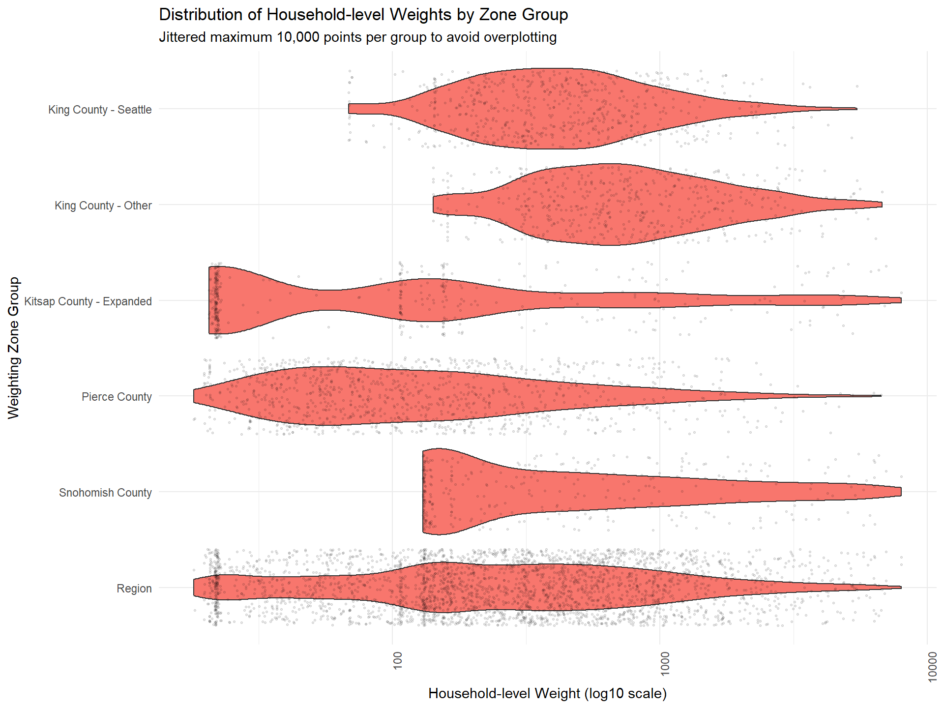
Figure: Fit Error (MAPE) Variance (CV) and Multimodality (DIP statistic) of Weights by Maximum Expansion Factor and Maximum Weight Cap
This diagnostic figure summarizes how fit error (MAPE), weight variance (CV), and multimodality (Dip Statistic) change as weighting parameters (maximum expansion factor, weight cap) are varied in PopulationSim. These metrics help balance the goals of matching ACS targets and maintaining stable, unimodal weight distributions.
- MAPE: Mean Absolute Percentage Error, measures discrepancy between weighted survey estimates and targets.
- CV: Coefficient of Variation, indicates weight variability.
- Dip Statistic: Measures the degree to which weights deviate from a single peak (unimodality).
Interpretation Note
Select weighting parameters where MAPE stabilizes, CV remains moderate, and Dip Statistic indicates unimodal distributions.
PSRC Specifics
Selecting a maximum weighting cap of 20,000 and expansion factor of 7 for PSRC is motivated by the balance displayed in the figure between model fit, stability, and sample variability. As shown, increasing the expansion factor generally reduces the fit error (MAPE) and Dip Statistic, indicating improved fit and sample representativeness. However, very low caps or low expansion factors produce larger errors and less stability. At an expansion factor of 7 and a weight cap of 20,000, the model achieves a low fit error and Dip statistic, with the coefficient of variation remaining acceptably stable across different cap values.
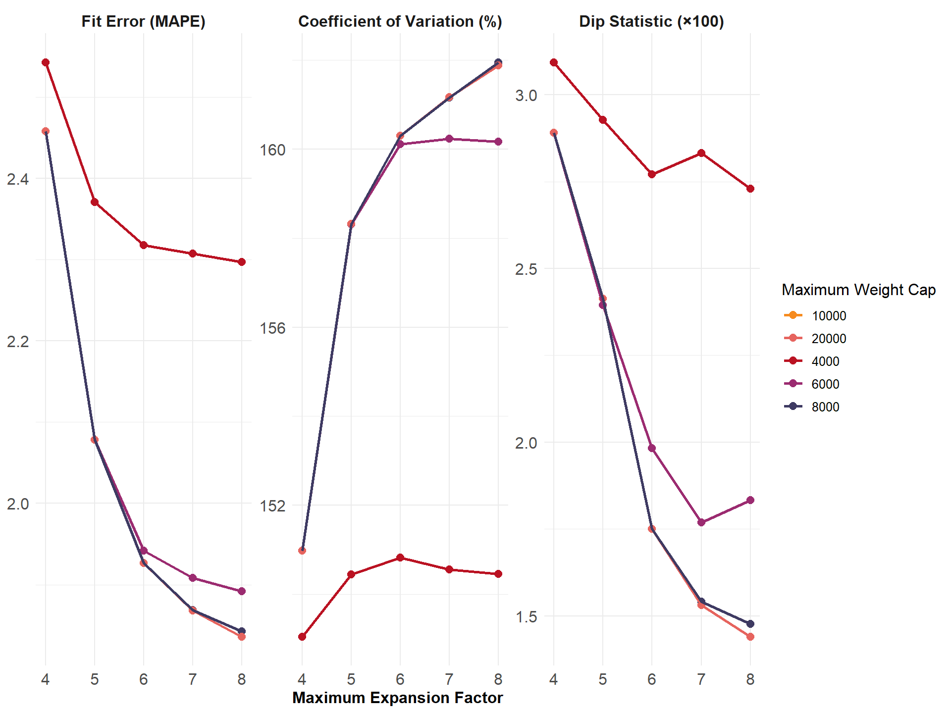
Table: Household- and Person-Level Weight Variability by Zone Group
The following table summarizes key variability statistics for the household- and person-level weights produced in Round 1. These statistics are calculated for each weighting zone group and for the region as a whole, using the maximum expansion factor applied in this weighting round.
- Household MAPE: Mean Absolute Percentage Error for household-level targets, indicating how closely weighted survey estimates match Census targets.
- Person MAPE: MAPE for person-level targets, showing fit to demographic controls.
- Coefficient of Variation: Standard deviation of weights divided by the mean, a normalized measure of weight variability.
Reviewing these metrics helps identify zones or groups where weights may be too variable or fit to targets may be weak.
Weighting zone group | N | Household MAPE | Person MAPE | Coefficient of variation |
|---|---|---|---|---|
King County - Seattle | 619 | 0.27 | 0.26 | 1.04 |
King County - Other | 518 | 0.25 | 0.18 | 0.99 |
Kitsap County - Expanded | 387 | 2.07 | 1.50 | 2.35 |
Pierce County | 1,050 | 0.22 | 0.21 | 1.98 |
Snohomish County | 336 | 1.06 | 0.79 | 1.56 |
Region | 2,910 | 0.46 | 0.38 | 1.61 |
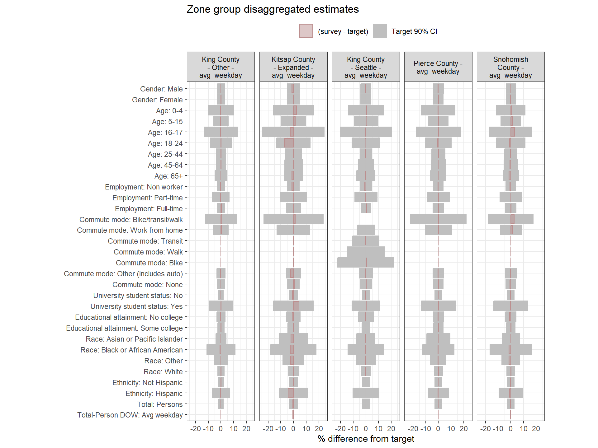
Round 1 Weight Fit to Targets
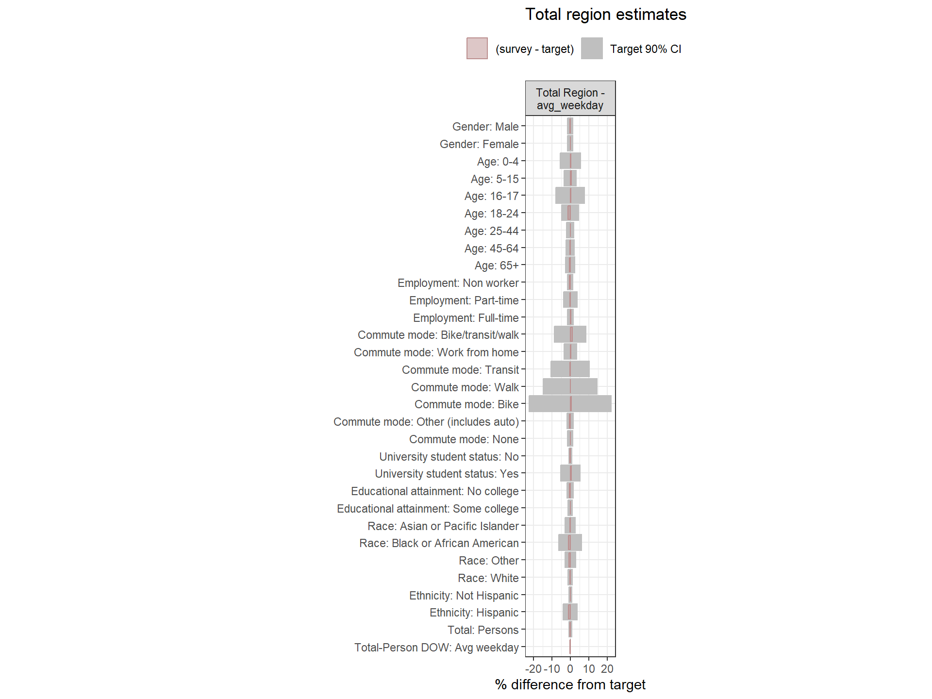
This section examines how well the weighted survey totals match the Census targets after Round 1 weighting. Each chart visualizes the percent difference between the weighted estimate and the target for each variable, alongside 90% confidence intervals around the target.
- Gray bars: 90% confidence interval as a percent of the target value.
- Red bars: Difference between the weighted survey estimate and the target. Negative bars indicate survey totals below the target.
If the red bar exceeds the confidence interval or if the interval itself is wide, this is a sign that the weighting approach may need adjustment. Red bars are bolded when error bounds are larger than desired (+/- 20% for regional estimates, +/- 25% for zone group estimates).
Weighting lever: Aggregate target categories
If some target categories or survey counts are very small, wide error margins may occur. Aggregating categories within certain zone groups or across the region can help minimize weight variance and produce more stable results. This should be considered after first adjusting weighting parameters.
Regional Weights Fit to Target Data
Figure: Household-Level Round 1 Weights Versus Target Estimates, by Day-of-Week
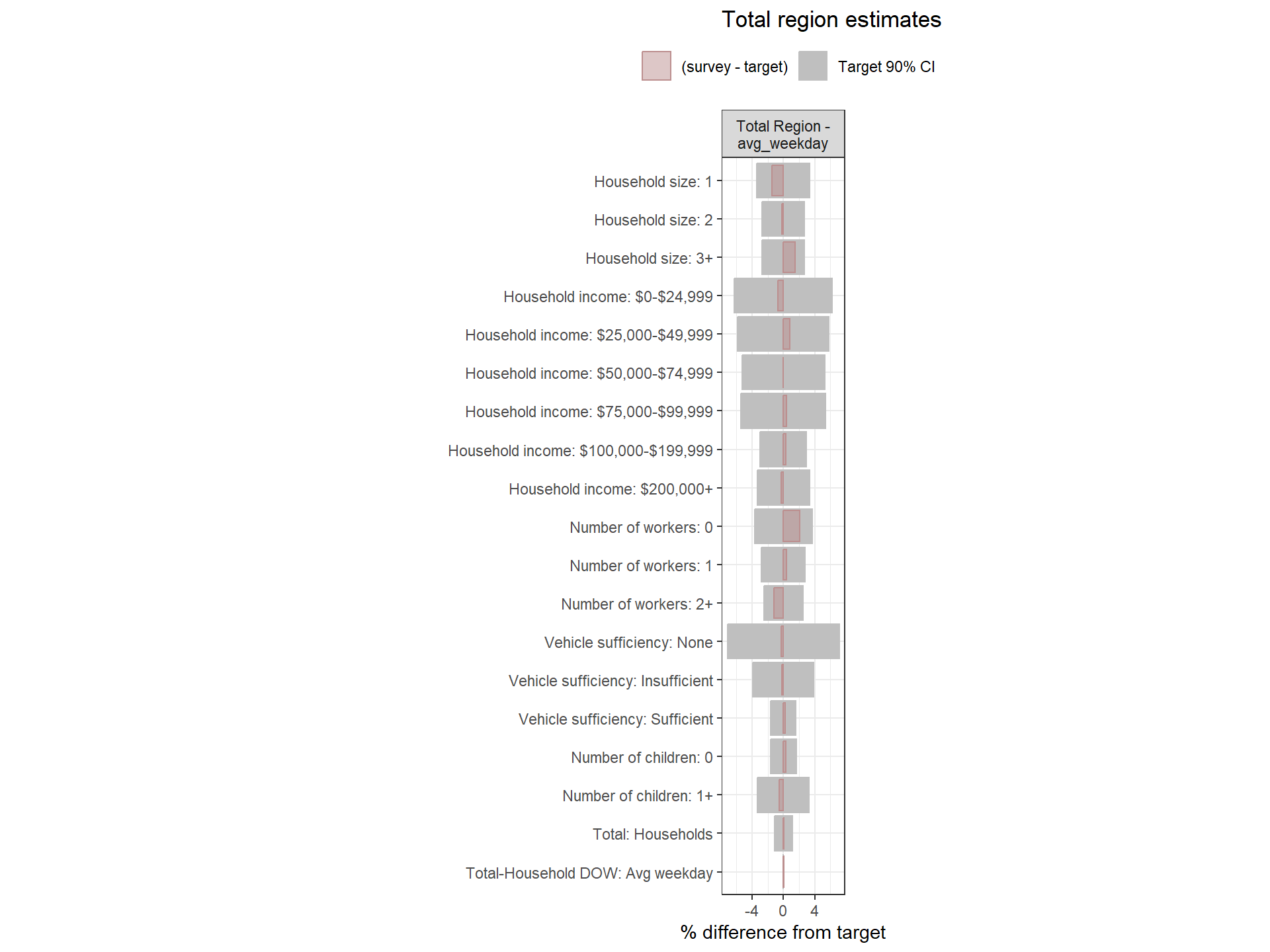
Figure: PUMA-Level Round 1 weights Versus Target Estimates, by Day-of-Week
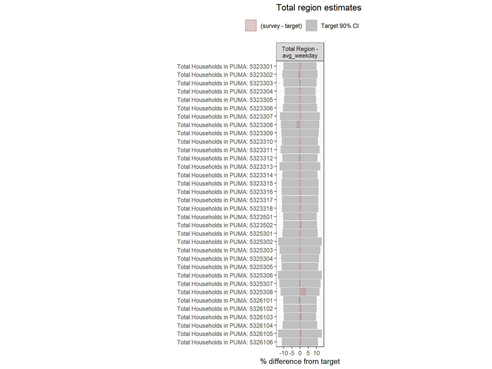
Figure: Person-Level Round 1 Weights Versus Target Estimates, by Day-of-Week
Weighting Zone Group Weights Fit to Target Data
Figure: Household-Level Round 1 Weights Versus Target Estimates, by Day-of-Week
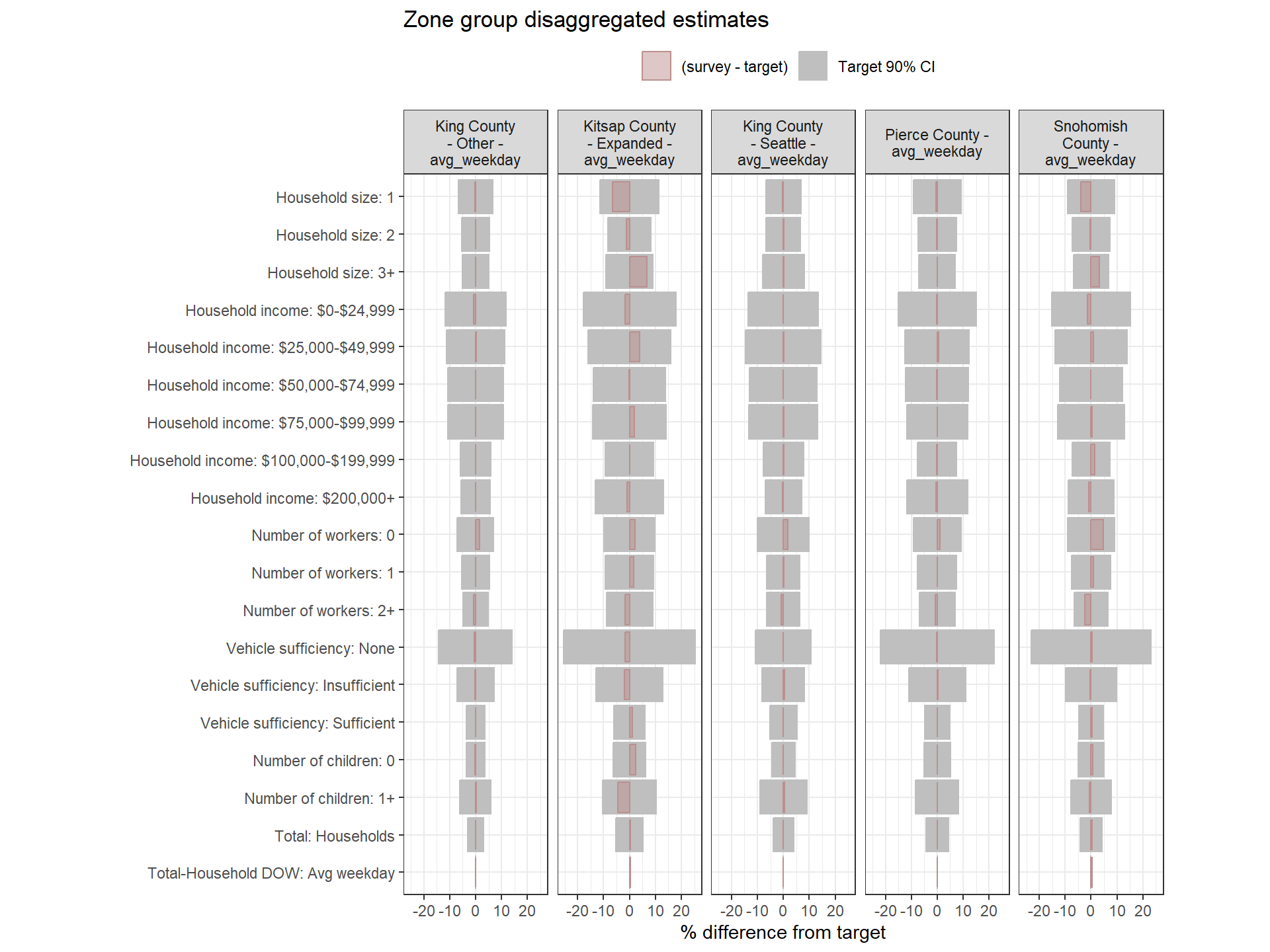
Figure: PUMA-Level Round 1 Weights Versus Target Estimates, by Day-of-Week
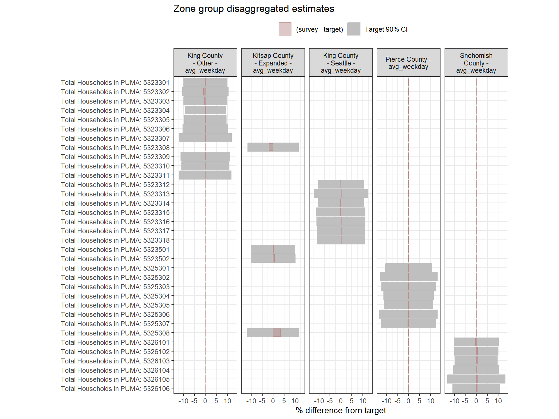
Figure: Person-Level Round 1 Weights Versus Target Estimates, by Day-of-Week