# Setup Environment
devtools::load_all()
settings = get_settings(reload_settings = TRUE,
                        print = FALSE)

# Params
code_root = get("code_root", settings)
work_dir = get('working_dir', settings)
inputs_dir = get('inputs_dir', settings)
outputs_dir = get('outputs_dir', settings)
report_dir = get('report_dir', settings)
popsim_initial_label = get("popsim_initial_label", settings)
popsim_daypat_label = get("popsim_daypat_label", settings)
run_label = get("popsim_daypat_label", settings)
popsim_dir <- file.path(work_dir, run_label)9 Round 2 Weighting: Day-Pattern Adjustments
9.1 Overview
This chapter describes the methods and processes used to implement Round 2 of the HTS weighting procedure: Day-Pattern Weighting. This step adjusts for differences in travel reporting by diary method (smartphone app, web-based diary, call center diary) using a model-based approach coupled with reweighting in PopulationSim. The output of this step is final household, person, and day weights that account for demographic nonresponse bias (Round 1) and day-pattern reporting bias (Round 2). These weights are then used as inputs to Round 3: Trip Weight Adjustment.
Many HTS projects with travel data collected via smartphone app typically exhibits higher trip rates compared to data collected via web or call center diary methods. There are three main reasons for this trend.
Households that own smartphones have different socio-demographic characteristics than households that do not own smartphones. These characteristics can correspond to higher trip-making activity.
Households that report their travel by smartphone tend to report fewer “stay at home” days. This may be due to the lower burden to recall trips when an app is tracking travel as it occurs.
On days with reported trips, households that report by smartphone tend to report an average higher number of trips for the reasons previously stated.
These three factors are interrelated and therefore must be isolated in any analysis and weighting adjustments. This process applies a two-stage approach to address differences in trip reporting across diary methods. In Round 2, adjusted weights at the person-day level are used to account for biases in day-pattern types; this step produces the final household, person and day weights. In Round 3, adjusted weights at the trip level are used, producing final linked trip, unlinked trip, and tour weights.
9.2 Chapter Setup
The day-pattern adjustment process requires many inputs, including the previously cleaned imputed and survey data; the base weights (in seed_wtd); demographic target data; and Round 1 household weights for QA/QC purposes. The code below loads these inputs and prepares them for use in the day-pattern modeling and weighting process.
Set Up Environment
First, we establish the environment and load some common parameters.
Load HTS Data
Next, we load the HTS data and codebook. The household and person files are the cleaned, post-imputation versions saved in earlier steps. The day and trip files are unmodified HTS tables.
# Codebook
variable_list = fetch_hts_table("variable_list", settings)
value_labels = fetch_hts_table("value_labels", settings)

# HTS Data with Imputations
households = readRDS(file.path(work_dir, 'households_survey_imputed.rds'))
persons = readRDS(file.path(work_dir, 'persons_survey_imputed.rds'))
days = fetch_hts_table("day", settings)
trips = fetch_hts_table("trip", settings)
Designate Source Table for Day-Pattern Counts
This stage re-loads either the unlinked or linked trip tables, depending on the value assigned to the setting daypat_adjustments_table.
Should I use unlinked or linked trips for day-pattern adjustments?
Users control whether the unlinked trip or linked trip table is used for day-pattern adjustments with the setting daypat_adjustments_table. The difference in the two tables is in the way transit are handled. The unlinked trip table contain separate records (rows) for the access and egress portions of transit trips, and in some cases, separate legs of a multi-transfer transit journey. The linked trip table stitches these legs into single journeys. Unlinked trips will have a high number of “change mode” trips, which get classified into “other” trips. If available, RSG recommends using the linked trip table, rather than the unlinked trip table, for day-pattern adjustments.
# Day Pattern Adjustment Table (Either Trip or Linked Trip)
daypat_table_type = settings$daypat_adjustments_table
if (is.null(daypat_table_type)) {
    stop("daypat_adjustments_table not set in settings")
} else{
  cli::cli_inform(paste0("Using ", daypat_table_type, " for day pattern adjustments"))
  daypat_table = fetch_hts_table(daypat_table_type, settings)
}
Filter to Valid Households
A safeguard is applied to ensure that only valid households (those present in the household file) are included in the day, trip, and day-pattern tables.
# Filter to Valid Household IDs
days = days[hh_id %in% households[, hh_id]]
trips = trips[hh_id %in% households$hh_id]
daypat_table = daypat_table[hh_id %in% households[, hh_id]]

# Add day_id to daypat_table if Missing, Joining via linked_trip_id
if (!"day_id" %in% colnames(daypat_table)) {
    daypat_table[trips, i.day_id, on = "linked_trip_id"]
}
Load Base Weights and Demographic Targets
Base weights (seed_wtd) and demographic targets are loaded. These form the backbone of the inputs to the second round of PopulationSim.
# Base Weights and Targets for PopulationSim
seed_wtd = readRDS(file.path(work_dir, 'survey_initial_wts.rds'))
targets_czone = readRDS(get("target_czone_path", settings))
targets_region = readRDS(get("target_region_path", settings))
Load Round 1 Household Weights
Round 1 household weights are loaded for use in the day-pattern modeling process (creating weighted generalized linear models for estimation).
# Read Household-Level Weights, Renaming the Weight Column for Consistency
hh_weights_path = file.path(
  work_dir,
  get('popsim_initial_label', settings),
  'output/final_summary_hh_weights.csv'
)

hh_weights = fread(hh_weights_path)
setnames(hh_weights, 'zone_group_balanced_weight', 'hh_weight')
9.3 Day-Pattern Modeling
This step uses a multinomial log-linear model (“choice model”) to estimate the probability of each day type (no trips, made mandatory trips, made non-mandatory trips) for each person-day. These model estimates are used to create new day-pattern targets for the second round of PopulationSim.
In development
Future versions of the day-pattern model may draw on external household travel surveys to improve stability and generalizability; pooling data across multiple regions would allow the model to capture a wider range of behavioral and reporting patterns than a single survey can represent. The goal of this work is to improve cross-survey consistency in day-pattern adjustments and reduce the need to re-estimate the model for each individual study.
Prepare Data for Day-Pattern Modelling
Minor Fixes
This code performs a couple of specific fixes on the daypat_table prior to modeling. Note, this will not change the existing trip or linked_trip table.
# Convert Dependent Variable to Character for Modeling
daypat_table[, d_purpose_category := as.character(d_purpose_category)]

## PSRC-Specific Fixes: Change Loop Trips to Other, Drop Missing d_purpose_category for daypat Adjustment Model
# Correct PSRC-Specific Coding Issues and Remove Missing Categories
daypat_table[d_purpose_category == 14, d_purpose_category := 13]
daypat_table <- daypat_table[d_purpose_category != 995]
Classify Person-Days into Day-Type Categories
This step leverages function calc_day_trip_class to classify person-days into four mutually exclusive and exhaustive day-type categories:
- Made no trips: The person made no trips on the day.
- Made mandatory trips: The person made trips to or from “work,” “work-related,” “school” or “school-related” activities.
- Made non-mandatory trips only: The person made one or more trips, but none were to or from “work,” “work-related,” “school” or “school-related” activities.
- Children’s trips: These trips are those reported by proxy for those under 18, regardless of the day-type category.
Children’s travel days
Children’s travel days are currently counted separately; because children’s trips are reported by proxy, this round of weighting does not adjust for potential reporting bias among child respondents. This approach avoids compounding uncertainty from proxy reporting and focuses adjustments on self-reported travel. However, this assumption may change in future applications; improvements in proxy reporting protocols or imputation methods could allow children’s travel days to be included in the day-pattern adjustment alongside adult records.
day_classes = calc_day_trip_class(daypat_table, daypat_table_type, days, value_labels)

dplyr::glimpse(day_classes)
Rows: 11,647
Columns: 6
$ hh_id <chr> "25000006", "25000006", "25000071", "25000096", "25000…
$ person_id <chr> "2500000601", "2500000602", "2500007101", "2500009601"…
$ day_id <chr> "250000060101", "250000060201", "250000710101", "25000…
$ travel_dow <dbl> 1, 1, 1, 4, 4, 4, 2, 2, 4, 4, 2, 2, 2, 2, 1, 1, 1, 2, …
$ day_trip_class <fct> none, none, non-mandatory, mandatory, none, non-mandat…
$ hh_day_complete <dbl> 1, 1, 1, 1, 1, 1, 1, 1, 1, 1, 1, 1, 1, 1, 1, 1, 1, 1, …Filter to Complete, Weighting-Eligible Days
This chunk filters the person-day dataset to include only complete household-days and eligible travel days (weighted days only). It then saves the classified day types to a CSV file for use in reporting.
# Drop Days Excluded from Day Groups (Weighted Days Only)
day_groups = get_day_groups(settings)
day_classes[day_groups, day_group := i.day_group, on = "travel_dow"]
day_classes = day_classes[!is.na(day_group)]

# Add daygroup to Days
days[day_groups, day_group := i.day_group, on = "travel_dow"]

# Drop Incomplete Days
day_classes = day_classes[hh_day_complete == 1,]

# Save File for Outputs
fwrite(day_classes, file.path(get("working_dir", settings), "day_classes.csv"))
Prepare Household-Level Variables for Modeling
In this section, we create indicator variables for diary platform (online/browser and call center) and zero-vehicle households. We then merge these household-level variables into the person-day dataset for modeling (fit_dt).
# Verify Required Diary Platforms are Present in the Data
stopifnot(
    all(c("rmove", "browser", "call") %in% unique(households$diary_platform))
)

# Create Diary Mode Indicator Variables for Modeling
households[, diary_online := 1 * (diary_platform == 'browser')]
households[, diary_call := 1 * (diary_platform == 'call')]
households[, zero_vehicle := 1 * (num_vehicles == 0)]

# Restrict Day Classes to Valid Households
day_classes = day_classes[hh_id %in% households$hh_id]

# Merge day_classes and Household Variables for the Model Input Dataset
fit_dt = merge(
  day_classes,
  households[, .(hh_id, diary_platform, diary_online, diary_call, zero_vehicle, income_imputed_label, income_detailed)],
  by = "hh_id",
  all = TRUE
)

# Check for Missing Values in Key Model Variables
stopifnot(
#   fit_dt[is.na(income_imputed_label), .N] == 0,
  fit_dt[is.na(day_trip_class), .N] == 0
)

dplyr::glimpse(fit_dt)
Rows: 7,578
Columns: 13
$ hh_id <chr> "25000006", "25000006", "25000071", "25000096", "…
$ person_id <chr> "2500000601", "2500000602", "2500007101", "250000…
$ day_id <chr> "250000060101", "250000060201", "250000710101", "…
$ travel_dow <dbl> 1, 1, 1, 4, 4, 4, 2, 2, 4, 4, 2, 2, 2, 2, 1, 1, 1…
$ day_trip_class <fct> none, none, non-mandatory, mandatory, none, non-m…
$ hh_day_complete <dbl> 1, 1, 1, 1, 1, 1, 1, 1, 1, 1, 1, 1, 1, 1, 1, 1, 1…
$ day_group <chr> "avg_weekday", "avg_weekday", "avg_weekday", "avg…
$ diary_platform <chr> "browser", "browser", "browser", "browser", "brow…
$ diary_online <dbl> 1, 1, 1, 1, 1, 1, 1, 1, 1, 1, 1, 1, 1, 1, 1, 1, 1…
$ diary_call <dbl> 0, 0, 0, 0, 0, 0, 0, 0, 0, 0, 0, 0, 0, 0, 0, 0, 0…
$ zero_vehicle <dbl> 0, 0, 0, 0, 0, 0, 0, 0, 0, 0, 0, 0, 0, 0, 0, 0, 0…
$ income_imputed_label <fct> "$25,000 - $49,999", "$25,000 - $49,999", "$100,0…
$ income_detailed <int> 999, 999, 999, 7, 7, 7, 7, 7, 6, 6, 4, 4, 4, 4, 2…Prepare Person-Level Variables for Modeling
This chunk prepares person-level variables for day-pattern modeling. It creates age group indicators (adult, under 35, 65+), flags employment and student status, and merges these with the main modeling dataset. The code also filters out non-surveyable persons (e.g., for surveys that do not require travel diaries from non-relatives).
Warning
Important: Ensure that all pattern regular expression strings correctly match the intended labels in your dataset. Adjust these patterns as necessary based on your specific value labels.
Future versions of this toolkit may include a yaml settings-driven approach to specify these patterns.
# Prepare Age Categories and Indicators for Adults, Under 35, and 65+
age_adult = 18

age_dt = value_labels[variable == "age", .(age = value, label)]
age_dt[, age_ub := get_age_upper_bounds(label)]
age_dt[,
  age_ub := fifelse(is.na(age_ub), max(age_ub, na.rm = TRUE) + 1, age_ub)
]

age_dt[, age_under_35 := 1 * (age_ub < 35)]
age_dt[, age_over_65 := 1 * (age_ub >= 65)]
age_dt[, is_adult := 1 * (age_ub >= age_adult)]
age_dt[, age := as.integer(age)]

# Add Age Indicators to Persons Data
persons = merge(
  persons,
  age_dt,
  by = "age",
  all.x = TRUE
)

# Mark Adults in day_classes for Further Filtering
day_classes[persons, is_adult := i.is_adult, on = "person_id"]

# Remove Nonrelatives from Model Input Dataset if Specified in Settings
if (settings$unrelated_adjustment != "none") {

  # Identify unrelated persons
  pattern = "nonrelative|unrelated|household help|roommate/friend|^other$"

  # Drop non-surveyable persons
  relationship_unrelated = value_labels[
    variable == 'relationship' &
      str_detect(str_to_lower(label), pattern),
    value
  ]

  stopifnot(
    persons[
      !(person_id %in% days$person_id) &
        is_complete == 1 &
        !(relationship %in% relationship_unrelated),
      .N
    ] ==
      0
  )
}

# Set Employment and Student Indicators for Modeling
nonworking_vals = value_labels[
  variable == "employment" &
    !label %like% "Employed full|Employed part|Self-employed|Missing",
  value
]

student_vals = value_labels[
  variable == "student" & label %like% "(?i)(Full|Part)-time student",
  value
]

uni_vals = value_labels[
  variable == "school_type" & label %like% "(?i)college|graduate|university",
  value
]

# is_employed
persons[, is_employed := ifelse(!employment %in% nonworking_vals, 1, 0)]

# is_student
persons[,
  is_student := ifelse(
    school_type %in% uni_vals & student %in% student_vals,
    1,
    0
  )
]

# Merge Person Variables into Model Input Dataset
n_fit = fit_dt[, .N]

fit_dt[, person_id := as.character(person_id)]

fit_dt = merge(
  fit_dt,
  persons[, .(
    person_id,
    is_adult,
    age_under_35,
    age_over_65,
    is_employed,
    is_student
  )],
  by = "person_id",
  all.x = TRUE
)

# Confirm that Age Variables are Not Missing After Merge
stopifnot(
  fit_dt[is.na(age_under_35), .N] == 0,
  fit_dt[, .N] == n_fit
)

# Ensure All Eligible Adults are Included in the Model Input Data
if (settings$unrelated_adjustment != "none") {
  stopifnot(
    persons[
      (!relationship %in% relationship_unrelated) &
        is_complete == 1 &
        is_adult == 1 &
        (hh_id %in% households$hh_id) &
        !(person_id %in% fit_dt[, person_id]),
      .N
    ] ==
      0
  )
} else {
   stopifnot(
    persons[
        is_complete == 1 &
        is_adult == 1 &
        (hh_id %in% households$hh_id) &
        !(person_id %in% fit_dt[, person_id]),
      .N
    ] ==
      0
  )
}

dplyr::glimpse(fit_dt)
Rows: 7,578
Columns: 18
$ person_id <chr> "2500000601", "2500000602", "2500007101", "250000…
$ hh_id <chr> "25000006", "25000006", "25000071", "25000096", "…
$ day_id <chr> "250000060101", "250000060201", "250000710101", "…
$ travel_dow <dbl> 1, 1, 1, 4, 4, 4, 2, 2, 4, 4, 2, 2, 2, 2, 1, 1, 1…
$ day_trip_class <fct> none, none, non-mandatory, mandatory, none, non-m…
$ hh_day_complete <dbl> 1, 1, 1, 1, 1, 1, 1, 1, 1, 1, 1, 1, 1, 1, 1, 1, 1…
$ day_group <chr> "avg_weekday", "avg_weekday", "avg_weekday", "avg…
$ diary_platform <chr> "browser", "browser", "browser", "browser", "brow…
$ diary_online <dbl> 1, 1, 1, 1, 1, 1, 1, 1, 1, 1, 1, 1, 1, 1, 1, 1, 1…
$ diary_call <dbl> 0, 0, 0, 0, 0, 0, 0, 0, 0, 0, 0, 0, 0, 0, 0, 0, 0…
$ zero_vehicle <dbl> 0, 0, 0, 0, 0, 0, 0, 0, 0, 0, 0, 0, 0, 0, 0, 0, 0…
$ income_imputed_label <fct> "$25,000 - $49,999", "$25,000 - $49,999", "$100,0…
$ income_detailed <int> 999, 999, 999, 7, 7, 7, 7, 7, 6, 6, 4, 4, 4, 4, 2…
$ is_adult <dbl> 1, 1, 1, 1, 1, 1, 1, 1, 1, 1, 1, 1, 1, 0, 1, 1, 1…
$ age_under_35 <dbl> 0, 0, 0, 0, 0, 0, 0, 0, 0, 0, 0, 0, 0, 1, 0, 0, 0…
$ age_over_65 <dbl> 1, 1, 1, 0, 1, 0, 0, 1, 1, 1, 0, 0, 0, 0, 0, 1, 1…
$ is_employed <dbl> 1, 1, 1, 1, 1, 1, 1, 1, 1, 1, 1, 1, 1, 1, 1, 1, 1…
$ is_student <dbl> 0, 0, 0, 0, 0, 0, 0, 0, 0, 0, 0, 0, 0, 0, 0, 0, 0…Create Model Estimation Weights
To account for multi-day travel diary data, avoid over-representation of rMove data in the model estimation, and verify the model estimates reflected population behavior (rather than the behavior of the sample), the model was weighted using Round 1 day weights scaled (divided) by the mean of the day weight across all days in the estimation dataset.
This normalization enforces that:
The relative influence of each record was preserved (households with larger day weights still had greater influence).
The average weight equaled 1, preventing the total weight from inflating model likelihoods or convergence behavior.
The effective sample size of the weighted dataset was similar to the unweighted number of observations, producing more stable coefficient estimates and variance calculations.
This approach is standard practice in weighted regression when model estimation is sensitive to large variations in survey weights.
The code below calculates these estimation weights and merges them into the model input dataset (fit_dt).
# --- Estimation Weights ---

# Calculate the Number of Complete Weekdays per Household for Normalization
hh_complete_days = calc_complete_hhdays(households, settings = settings, days = days)

hh_complete_days[, hh_id := as.character(hh_id)]

# Add in the Day Group and Original hh_id to the Weights
hh_weights[seed_wtd, `:=`(hh_id = i.hh_id, day_group = i.day_group), on = "hh_id_dow"]
hh_weights[hh_complete_days, n_complete_hh_days := i.n_complete_hh_days, on = .(hh_id_dow)]
hh_weights[households, `:=`(
        num_people = i.num_people,
        num_adults = i.num_adults
    ), on = .(hh_id)
]

# Calculate Person-Level Weights
person_weights = calc_person_weights(
    hh_weights,
    households,
    persons,
    value_labels,
    settings
)

# Calculate Day-Level Weights
day_weights = calc_day_weights(
    person_weights,
    households,
    persons,
    days,
    trips,
    value_labels,
    settings
)

# Normalize Day Weights so that Model Standard Errors are Meaningful
fit_dt[day_weights, day_weight := i.day_weight, on = "day_id"]
fit_dt[, estimation_weight := day_weight / mean(day_weight)]

dplyr::glimpse(fit_dt)
Rows: 7,578
Columns: 20
$ person_id <chr> "2500000601", "2500000602", "2500007101", "250000…
$ hh_id <chr> "25000006", "25000006", "25000071", "25000096", "…
$ day_id <chr> "250000060101", "250000060201", "250000710101", "…
$ travel_dow <dbl> 1, 1, 1, 4, 4, 4, 2, 2, 4, 4, 2, 2, 2, 2, 1, 1, 1…
$ day_trip_class <fct> none, none, non-mandatory, mandatory, none, non-m…
$ hh_day_complete <dbl> 1, 1, 1, 1, 1, 1, 1, 1, 1, 1, 1, 1, 1, 1, 1, 1, 1…
$ day_group <chr> "avg_weekday", "avg_weekday", "avg_weekday", "avg…
$ diary_platform <chr> "browser", "browser", "browser", "browser", "brow…
$ diary_online <dbl> 1, 1, 1, 1, 1, 1, 1, 1, 1, 1, 1, 1, 1, 1, 1, 1, 1…
$ diary_call <dbl> 0, 0, 0, 0, 0, 0, 0, 0, 0, 0, 0, 0, 0, 0, 0, 0, 0…
$ zero_vehicle <dbl> 0, 0, 0, 0, 0, 0, 0, 0, 0, 0, 0, 0, 0, 0, 0, 0, 0…
$ income_imputed_label <fct> "$25,000 - $49,999", "$25,000 - $49,999", "$100,0…
$ income_detailed <int> 999, 999, 999, 7, 7, 7, 7, 7, 6, 6, 4, 4, 4, 4, 2…
$ is_adult <dbl> 1, 1, 1, 1, 1, 1, 1, 1, 1, 1, 1, 1, 1, 0, 1, 1, 1…
$ age_under_35 <dbl> 0, 0, 0, 0, 0, 0, 0, 0, 0, 0, 0, 0, 0, 1, 0, 0, 0…
$ age_over_65 <dbl> 1, 1, 1, 0, 1, 0, 0, 1, 1, 1, 0, 0, 0, 0, 0, 1, 1…
$ is_employed <dbl> 1, 1, 1, 1, 1, 1, 1, 1, 1, 1, 1, 1, 1, 1, 1, 1, 1…
$ is_student <dbl> 0, 0, 0, 0, 0, 0, 0, 0, 0, 0, 0, 0, 0, 0, 0, 0, 0…
$ day_weight <dbl> 31.09526, 31.09526, 99.16948, 22.09291, 22.09291,…
$ estimation_weight <dbl> 0.05558718, 0.05558718, 0.17727948, 0.03949420, 0…Filter to Adults
The last step before estimating the day-pattern model is to filter the dataset to adults only, as children’s travel is reported by proxy and may exhibit different reporting biases. The code below performs this filtering.
# Filter Dataset to Adults Only for Modeling
fit_dt = fit_dt[is_adult == 1]
dplyr::glimpse(fit_dt)
Rows: 6,707
Columns: 20
$ person_id <chr> "2500000601", "2500000602", "2500007101", "250000…
$ hh_id <chr> "25000006", "25000006", "25000071", "25000096", "…
$ day_id <chr> "250000060101", "250000060201", "250000710101", "…
$ travel_dow <dbl> 1, 1, 1, 4, 4, 4, 2, 2, 4, 4, 2, 2, 2, 1, 1, 1, 2…
$ day_trip_class <fct> none, none, non-mandatory, mandatory, none, non-m…
$ hh_day_complete <dbl> 1, 1, 1, 1, 1, 1, 1, 1, 1, 1, 1, 1, 1, 1, 1, 1, 1…
$ day_group <chr> "avg_weekday", "avg_weekday", "avg_weekday", "avg…
$ diary_platform <chr> "browser", "browser", "browser", "browser", "brow…
$ diary_online <dbl> 1, 1, 1, 1, 1, 1, 1, 1, 1, 1, 1, 1, 1, 1, 1, 1, 1…
$ diary_call <dbl> 0, 0, 0, 0, 0, 0, 0, 0, 0, 0, 0, 0, 0, 0, 0, 0, 0…
$ zero_vehicle <dbl> 0, 0, 0, 0, 0, 0, 0, 0, 0, 0, 0, 0, 0, 0, 0, 0, 0…
$ income_imputed_label <fct> "$25,000 - $49,999", "$25,000 - $49,999", "$100,0…
$ income_detailed <int> 999, 999, 999, 7, 7, 7, 7, 7, 6, 6, 4, 4, 4, 2, 2…
$ is_adult <dbl> 1, 1, 1, 1, 1, 1, 1, 1, 1, 1, 1, 1, 1, 1, 1, 1, 1…
$ age_under_35 <dbl> 0, 0, 0, 0, 0, 0, 0, 0, 0, 0, 0, 0, 0, 0, 0, 0, 0…
$ age_over_65 <dbl> 1, 1, 1, 0, 1, 0, 0, 1, 1, 1, 0, 0, 0, 0, 1, 1, 1…
$ is_employed <dbl> 1, 1, 1, 1, 1, 1, 1, 1, 1, 1, 1, 1, 1, 1, 1, 1, 1…
$ is_student <dbl> 0, 0, 0, 0, 0, 0, 0, 0, 0, 0, 0, 0, 0, 0, 0, 0, 0…
$ day_weight <dbl> 31.09526, 31.09526, 99.16948, 22.09291, 22.09291,…
$ estimation_weight <dbl> 0.05558718, 0.05558718, 0.17727948, 0.03949420, 0…Estimate Day-Pattern Model
The day-pattern model is estimated using a weighted multinomial logistic regression. The model predicts the day-type class for each person-day record based on demographic and diary platform variables, with interaction terms for diary platform and age groups. If multiple day groups are present, (e.g., weekdays and weekends), the model includes interactions with day_group to capture variations in travel behavior across different days of the week.
Prepare Model Formula
The model formula is dynamically constructed based on the variables specified in the settings file. This allows for flexibility in modifying the model without changing the code directly. Users can adjust the setting daypat_formula_vars setting to include or exclude variables as needed.
In Development: Model type
The current multinomial logit framework is intentionally simple, but alternative approaches such as machine-learning classifiers may be explored to better capture non-linear relationships between demographics, household context, and diary method.
In Development: Alternative specifications for day_group interaction
Commented-out code in the chunk below provides alternative specifications for how to include day_group in the model:
- Simple fixed effect with day_group
- Full separation by day_group
- Full interaction with day_group (currently used)
These model formulations can be tested and compared based on model fit statistics and predictive performance. Note, this area of code is in development and may be updated in future versions of the toolkit.
# Dynamically Build the Model Formula from Variables Set in Settings
formula_vars = get("daypat_formula_vars", settings)
model_formula = as.formula(paste("day_trip_class ~", paste(formula_vars, collapse = " + ")))

# If More Than One day_group, Add day_group to the Model
# DOW Provides Better Predictive Power When Spanning Weekends
if (length(get("weight_dow_groups", settings)) > 1) {
    # Extract the response and term labels
    response = all.vars(model_formula)[1]
    terms_list = attr(terms(model_formula), "term.labels")

    # Collapse the terms into a string
    rhs = paste(terms_list, collapse = " + ")

    # Wrap the RHS in parentheses and add interaction with 'day_group'

    # Simple fixed effect with day_group
    # rhs_interacted = paste("day_group + (", rhs, ")")

    # Full separation by day_group
    # rhs_interacted = paste("0 + day_group : (", rhs, ")")

    # Full interaction with day_group
    rhs_interacted = paste("day_group * (", rhs, ")")

    # Rebuild the formula
    model_formula = as.formula(paste(response, "~", rhs_interacted))
}

cli::cli_inform(c("Model formula: ", model_formula))
Fit Day-Pattern Model
This chunk fits the weighted multinomial logistic regression model using the prepared dataset and estimation weights. An internal function, check_daypat_results, checks that observed and predicted estimates are equal for model fit. McFadden’s R^2 is then calculated to assess model fit.
# Fit a Weighted Multinomial Logistic Regression Model to Predict Day Trip Class
model = multinom(
  model_formula,
  data = fit_dt,
  weights = fit_dt[, estimation_weight],
  model = TRUE,
  Hess = 1000,
  trace = FALSE # Set this to TRUE for viewing outputs for model convergence
)

# Compare Observed and Predicted Shares to Check Model Fit
check_daypat_results(model, fit_dt)

# Calculate Model Coefficients and Diagnostics for Review
mdl <- broom::tidy(model, exponentiate = FALSE)
rho2 <- DescTools::PseudoR2(model)
Save Model Results
Model coefficients and fit are then saved for review.
# Save Model Results for Use in Reporting and Further Analysis
report_dir = get('report_dir', settings)

fwrite(
  mdl,
  file.path(report_dir, "models", "day_pattern_model_coef.csv")
)

fwrite(
  as.data.table(rho2),
  file.path(report_dir, "models", "day_pattern_model_fit.csv")
)
Table: Day Pattern Model Summary
Alternative | Variable | Estimate | Std Error | T-Statistic | p.value |
|---|---|---|---|---|---|
mandatory1 | Model intercept | 0.893 | 0.076 | 11.76 | <0.001 |
Zero vehicle household | -0.564 | 0.167 | -3.37 | <0.001 | |
Income over $200,000+ | 0.049 | 0.095 | 0.52 | 0.606 | |
Income $25,000 - $49,999 | -0.349 | 0.126 | -2.77 | 0.006 | |
Income $50,000 - $74,999 | 0.348 | 0.135 | 2.58 | 0.01 | |
Income $75,000 - $99,999 | 0.293 | 0.132 | 2.22 | 0.026 | |
Income under $25,000 | -1.075 | 0.174 | -6.17 | <0.001 | |
Age < 35 years | -0.114 | 0.233 | -0.49 | 0.624 | |
Age > 65 years | -1.807 | 0.114 | -15.82 | <0.001 | |
Employed full/part/self | 0.893 | 0.076 | 11.76 | <0.001 | |
Full or part-time student | 1.589 | 0.582 | 2.73 | 0.006 | |
Online diary data | -0.643 | 0.151 | -4.26 | <0.001 | |
Call center diary data | -0.779 | 0.323 | -2.41 | 0.016 | |
Online diary data, age <35 | 0.006 | 0.248 | 0.02 | 0.982 | |
Call center diary, age >65 | 0.375 | 0.537 | 0.70 | 0.485 | |
non-mandatory1 | Model intercept | 0.541 | 0.077 | 6.99 | <0.001 |
Zero vehicle household | -0.111 | 0.150 | -0.74 | 0.457 | |
Income over $200,000+ | 0.026 | 0.099 | 0.26 | 0.791 | |
Income $25,000 - $49,999 | -0.073 | 0.125 | -0.58 | 0.561 | |
Income $50,000 - $74,999 | 0.447 | 0.135 | 3.30 | <0.001 | |
Income $75,000 - $99,999 | -0.106 | 0.141 | -0.75 | 0.452 | |
Income under $25,000 | -0.043 | 0.148 | -0.29 | 0.773 | |
Age < 35 years | 0.191 | 0.236 | 0.81 | 0.42 | |
Age > 65 years | 0.128 | 0.091 | 1.41 | 0.16 | |
Employed full/part/self | 0.541 | 0.077 | 6.99 | <0.001 | |
Full or part-time student | 1.704 | 0.594 | 2.87 | 0.004 | |
Online diary data | -0.534 | 0.153 | -3.48 | <0.001 | |
Call center diary data | -0.608 | 0.313 | -1.94 | 0.052 | |
Online diary data, age <35 | -0.524 | 0.254 | -2.06 | 0.039 | |
Call center diary, age >65 | 0.116 | 0.422 | 0.27 | 0.783 | |
McFadden's rho-squared: 0.07 | |||||
1Alternatives are compared to making no trips | |||||
9.4 Update Seed and Targets
This section applies the day pattern model to the seed data to calculate the day pattern targets.
Update Seed
First, the observed day pattern shares are calculated and input as the initial day pattern targets with function update_daypat_seed. This function:
- Tabulates day pattern data to get average probabilities by household.
- Normalizes by number of days, not persons per household.
- Factors up probabilities by persons/surveyable ratio to match p_total.
The seed_wtd dataset is displayed below for reference.
dplyr::glimpse(seed_wtd)Rows: 2,910
Columns: 95
$ segment_name <chr> "King County-General", "King County-General",…
$ invitation <chr> "ABS", "ABS", "ABS", "ABS", "ABS", "ABS", "AB…
$ day_group <chr> "avg_weekday", "avg_weekday", "avg_weekday", …
$ hh_id <chr> "25011433", "25011496", "25011506", "25011518…
$ puma_id <chr> "5323318", "5323304", "5323318", "5323301", "…
$ client_zone_id <chr> "5323318", "5323304", "5323318", "5323301", "…
$ h_size_0_1 <dbl> 1, 1, 1, 0, 0, 1, 1, 0, 0, 0, 0, 1, 1, 0, 0, …
$ h_size_2 <dbl> 0, 0, 0, 0, 1, 0, 0, 0, 1, 1, 1, 0, 0, 1, 1, …
$ h_size_3_plus <dbl> 0, 0, 0, 1, 0, 0, 0, 1, 0, 0, 0, 0, 0, 0, 0, …
$ h_income_0_24999 <dbl> 0, 0, 0, 0, 0, 0, 0, 0, 0, 0, 0, 0, 0, 0, 0, …
$ h_income_25000_49999 <dbl> 0, 0, 1, 0, 0, 0, 0, 0, 0, 0, 0, 0, 0, 0, 0, …
$ h_income_50000_74999 <dbl> 0, 0, 0, 0, 0, 0, 0, 0, 0, 0, 0, 0, 0, 0, 0, …
$ h_income_75000_99999 <dbl> 0, 0, 0, 0, 0, 0, 0, 0, 0, 0, 1, 1, 0, 0, 0, …
$ h_income_100000_199999 <dbl> 1, 1, 0, 1, 0, 1, 1, 1, 1, 0, 0, 0, 1, 0, 1, …
$ h_income_200000_plus <dbl> 0, 0, 0, 0, 1, 0, 0, 0, 0, 1, 0, 0, 0, 1, 0, …
$ h_workers_0 <dbl> 0, 1, 1, 0, 0, 0, 1, 0, 0, 0, 0, 0, 1, 0, 1, …
$ h_workers_1 <dbl> 1, 0, 0, 0, 1, 1, 0, 0, 0, 0, 1, 1, 0, 1, 0, …
$ h_workers_2_plus <dbl> 0, 0, 0, 1, 0, 0, 0, 1, 1, 1, 0, 0, 0, 0, 0, …
$ h_vehicles_none <dbl> 0, 0, 1, 0, 0, 0, 0, 0, 0, 0, 0, 0, 0, 0, 0, …
$ h_vehicles_insuff <dbl> 0, 0, 0, 1, 0, 0, 0, 1, 0, 0, 1, 0, 0, 0, 0, …
$ h_vehicles_suff <dbl> 1, 1, 0, 0, 1, 1, 1, 0, 1, 1, 0, 1, 1, 1, 1, …
$ h_kids_0 <dbl> 1, 1, 1, 1, 1, 1, 1, 0, 1, 1, 1, 1, 1, 1, 1, …
$ h_kids_1_plus <dbl> 0, 0, 0, 0, 0, 0, 0, 1, 0, 0, 0, 0, 0, 0, 0, …
$ h_puma_5323301 <dbl> 0, 0, 0, 1, 0, 0, 0, 0, 0, 0, 1, 0, 0, 0, 0, …
$ h_puma_5323302 <dbl> 0, 0, 0, 0, 0, 0, 0, 0, 0, 0, 0, 0, 0, 0, 0, …
$ h_puma_5323303 <dbl> 0, 0, 0, 0, 1, 0, 0, 0, 0, 0, 0, 0, 0, 1, 1, …
$ h_puma_5323304 <dbl> 0, 1, 0, 0, 0, 0, 1, 0, 0, 1, 0, 0, 0, 0, 0, …
$ h_puma_5323305 <dbl> 0, 0, 0, 0, 0, 0, 0, 0, 0, 0, 0, 1, 0, 0, 0, …
$ h_puma_5323306 <dbl> 0, 0, 0, 0, 0, 0, 0, 0, 0, 0, 0, 0, 0, 0, 0, …
$ h_puma_5323307 <dbl> 0, 0, 0, 0, 0, 0, 0, 0, 0, 0, 0, 0, 0, 0, 0, …
$ h_puma_5323308 <dbl> 0, 0, 0, 0, 0, 0, 0, 0, 0, 0, 0, 0, 0, 0, 0, …
$ h_puma_5323309 <dbl> 0, 0, 0, 0, 0, 0, 0, 1, 0, 0, 0, 0, 0, 0, 0, …
$ h_puma_5323310 <dbl> 0, 0, 0, 0, 0, 0, 0, 0, 0, 0, 0, 0, 0, 0, 0, …
$ h_puma_5323311 <dbl> 0, 0, 0, 0, 0, 0, 0, 0, 0, 0, 0, 0, 0, 0, 0, …
$ h_puma_5323312 <dbl> 0, 0, 0, 0, 0, 0, 0, 0, 0, 0, 0, 0, 0, 0, 0, …
$ h_puma_5323313 <dbl> 0, 0, 0, 0, 0, 0, 0, 0, 0, 0, 0, 0, 0, 0, 0, …
$ h_puma_5323314 <dbl> 0, 0, 0, 0, 0, 0, 0, 0, 0, 0, 0, 0, 0, 0, 0, …
$ h_puma_5323315 <dbl> 0, 0, 0, 0, 0, 0, 0, 0, 0, 0, 0, 0, 1, 0, 0, …
$ h_puma_5323316 <dbl> 0, 0, 0, 0, 0, 0, 0, 0, 0, 0, 0, 0, 0, 0, 0, …
$ h_puma_5323317 <dbl> 0, 0, 0, 0, 0, 0, 0, 0, 0, 0, 0, 0, 0, 0, 0, …
$ h_puma_5323318 <dbl> 1, 0, 1, 0, 0, 1, 0, 0, 1, 0, 0, 0, 0, 0, 0, …
$ h_puma_5323501 <dbl> 0, 0, 0, 0, 0, 0, 0, 0, 0, 0, 0, 0, 0, 0, 0, …
$ h_puma_5323502 <dbl> 0, 0, 0, 0, 0, 0, 0, 0, 0, 0, 0, 0, 0, 0, 0, …
$ h_puma_5325301 <dbl> 0, 0, 0, 0, 0, 0, 0, 0, 0, 0, 0, 0, 0, 0, 0, …
$ h_puma_5325302 <dbl> 0, 0, 0, 0, 0, 0, 0, 0, 0, 0, 0, 0, 0, 0, 0, …
$ h_puma_5325303 <dbl> 0, 0, 0, 0, 0, 0, 0, 0, 0, 0, 0, 0, 0, 0, 0, …
$ h_puma_5325304 <dbl> 0, 0, 0, 0, 0, 0, 0, 0, 0, 0, 0, 0, 0, 0, 0, …
$ h_puma_5325305 <dbl> 0, 0, 0, 0, 0, 0, 0, 0, 0, 0, 0, 0, 0, 0, 0, …
$ h_puma_5325306 <dbl> 0, 0, 0, 0, 0, 0, 0, 0, 0, 0, 0, 0, 0, 0, 0, …
$ h_puma_5325307 <dbl> 0, 0, 0, 0, 0, 0, 0, 0, 0, 0, 0, 0, 0, 0, 0, …
$ h_puma_5325308 <dbl> 0, 0, 0, 0, 0, 0, 0, 0, 0, 0, 0, 0, 0, 0, 0, …
$ h_puma_5326101 <dbl> 0, 0, 0, 0, 0, 0, 0, 0, 0, 0, 0, 0, 0, 0, 0, …
$ h_puma_5326102 <dbl> 0, 0, 0, 0, 0, 0, 0, 0, 0, 0, 0, 0, 0, 0, 0, …
$ h_puma_5326103 <dbl> 0, 0, 0, 0, 0, 0, 0, 0, 0, 0, 0, 0, 0, 0, 0, …
$ h_puma_5326104 <dbl> 0, 0, 0, 0, 0, 0, 0, 0, 0, 0, 0, 0, 0, 0, 0, …
$ h_puma_5326105 <dbl> 0, 0, 0, 0, 0, 0, 0, 0, 0, 0, 0, 0, 0, 0, 0, …
$ h_puma_5326106 <dbl> 0, 0, 0, 0, 0, 0, 0, 0, 0, 0, 0, 0, 0, 0, 0, …
$ h_total <int> 1, 1, 1, 1, 1, 1, 1, 1, 1, 1, 1, 1, 1, 1, 1, …
$ p_gender_female <dbl> 0, 0, 1, 2, 1, 0, 0, 2, 1, 1, 1, 0, 1, 1, 1, …
$ p_gender_male <dbl> 1, 1, 0, 1, 1, 1, 1, 1, 1, 1, 1, 1, 0, 1, 1, …
$ p_age_0_4 <dbl> 0, 0, 0, 0, 0, 0, 0, 1, 0, 0, 0, 0, 0, 0, 0, …
$ p_age_5_15 <dbl> 0, 0, 0, 0, 0, 0, 0, 0, 0, 0, 0, 0, 0, 0, 0, …
$ p_age_16_17 <dbl> 0, 0, 0, 0, 0, 0, 0, 0, 0, 0, 0, 0, 0, 0, 0, …
$ p_age_18_24 <dbl> 0, 0, 0, 1, 0, 0, 0, 0, 0, 0, 0, 0, 0, 0, 0, …
$ p_age_25_44 <dbl> 0, 0, 1, 0, 0, 1, 0, 1, 2, 2, 2, 1, 0, 2, 0, …
$ p_age_45_64 <dbl> 0, 1, 0, 1, 2, 0, 0, 1, 0, 0, 0, 0, 0, 0, 0, …
$ p_age_65_plus <dbl> 1, 0, 0, 1, 0, 0, 1, 0, 0, 0, 0, 0, 1, 0, 2, …
$ p_employment_full_time <dbl> 1, 1, 0, 1, 1, 1, 1, 1, 2, 2, 1, 1, 1, 2, 0, …
$ p_employment_nonworker <dbl> 0, 0, 1, 1, 1, 0, 0, 1, 0, 0, 1, 0, 0, 0, 2, …
$ p_employment_part_time <dbl> 0, 0, 0, 1, 0, 0, 0, 1, 0, 0, 0, 0, 0, 0, 0, …
$ p_commutemode_bike <dbl> 0, 0, 0, 0, 0, 0, 0, 0, 0, 1, 0, 0, 0, 0, 0, …
$ p_commutemode_home <dbl> 0, 1, 0, 1, 1, 1, 1, 1, 1, 0, 1, 0, 1, 2, 0, …
$ p_commutemode_none <dbl> 0, 0, 1, 1, 1, 0, 0, 1, 0, 0, 1, 0, 0, 0, 2, …
$ p_commutemode_other <dbl> 1, 0, 0, 0, 0, 0, 0, 1, 1, 0, 0, 1, 0, 0, 0, …
$ p_commutemode_transit <dbl> 0, 0, 0, 0, 0, 0, 0, 0, 0, 1, 0, 0, 0, 0, 0, …
$ p_commutemode_walk <dbl> 0, 0, 0, 1, 0, 0, 0, 0, 0, 0, 0, 0, 0, 0, 0, …
$ p_univstudent_no <dbl> 1, 1, 1, 3, 2, 1, 1, 3, 1, 2, 2, 1, 1, 2, 2, …
$ p_univstudent_yes <dbl> 0, 0, 0, 0, 0, 0, 0, 0, 1, 0, 0, 0, 0, 0, 0, …
$ p_edulevel_no_college <dbl> 0, 0, 1, 1, 0, 0, 0, 1, 0, 0, 2, 1, 0, 0, 2, …
$ p_edulevel_some_college <dbl> 1, 1, 0, 2, 2, 1, 1, 2, 2, 2, 0, 0, 1, 2, 0, …
$ p_race_afam <dbl> 0, 0, 0, 0, 0, 0, 0, 0, 0, 0, 1, 0, 0, 0, 0, …
$ p_race_asian_pacific <dbl> 0, 1, 0, 1, 0, 1, 1, 1, 0, 1, 0, 0, 0, 1, 1, …
$ p_race_other <dbl> 0, 0, 0, 0, 0, 0, 0, 0, 0, 0, 0, 0, 0, 0, 0, …
$ p_race_white <dbl> 1, 0, 1, 2, 2, 0, 0, 2, 2, 1, 1, 1, 1, 1, 1, …
$ p_ethnicity_not_hispanic <dbl> 1, 1, 1, 3, 2, 1, 1, 3, 1, 2, 2, 1, 1, 2, 2, …
$ p_ethnicity_hispanic <dbl> 0, 0, 0, 0, 0, 0, 0, 0, 1, 0, 0, 0, 0, 0, 0, …
$ p_total <int> 1, 1, 1, 3, 2, 1, 1, 3, 2, 2, 2, 1, 1, 2, 2, …
$ region <dbl> 1, 1, 1, 1, 1, 1, 1, 1, 1, 1, 1, 1, 1, 1, 1, …
$ bg_geoid <chr> "530330012022", "530330233003", "530330011002…
$ h_dow_avg_weekday <int> 1, 1, 1, 1, 1, 1, 1, 1, 1, 1, 1, 1, 1, 1, 1, …
$ hh_id_dow <chr> "25011433_avg_weekday", "25011496_avg_weekday…
$ p_dow_avg_weekday <int> 1, 1, 1, 3, 2, 1, 1, 3, 2, 2, 2, 1, 1, 2, 2, …
$ zone_group <chr> "King County - Seattle", "King County - Other…
$ initial_weight <dbl> 1000.324, 1000.324, 1000.324, 1000.324, 1000.…
$ alpha <dbl> 1, 1, 1, 1, 1, 1, 1, 1, 1, 1, 1, 1, 1, 1, 1, …After updating, seed_daypat contains the observed day pattern shares for adults in the survey data, shown as p_made_mandatory_avg_weekday, p_made_nonmand_avg_weekday, p_made_none_avg_weekday, and p_made_child_avg_weekday:
# --- Update Seed and Targets ---
# Tabulate Observed Day Pattern Shares for Adults (Seed Data)
seed_daypat = update_daypat_seed(seed_wtd, day_classes, households, settings)

dplyr::glimpse(seed_daypat)
Rows: 2,910
Columns: 99
$ hh_id <chr> "25000006", "25000071", "25000096", "2500…
$ client_zone_id <chr> "5325306", "5325305", "5325308", "5325304…
$ h_size_0_1 <dbl> 0, 1, 0, 0, 0, 0, 0, 0, 1, 0, 0, 0, 1, 1,…
$ h_size_2 <dbl> 1, 0, 0, 1, 1, 0, 0, 0, 0, 1, 1, 0, 0, 0,…
$ h_size_3_plus <dbl> 0, 0, 1, 0, 0, 1, 1, 1, 0, 0, 0, 1, 0, 0,…
$ h_income_0_24999 <dbl> 0, 0, 0, 0, 0, 0, 1, 0, 0, 0, 0, 0, 0, 0,…
$ h_income_25000_49999 <dbl> 1, 0, 0, 0, 0, 1, 0, 1, 0, 0, 0, 0, 0, 0,…
$ h_income_50000_74999 <dbl> 0, 0, 0, 0, 0, 0, 0, 0, 1, 1, 0, 0, 1, 0,…
$ h_income_75000_99999 <dbl> 0, 0, 0, 0, 1, 0, 0, 0, 0, 0, 0, 0, 0, 1,…
$ h_income_100000_199999 <dbl> 0, 1, 1, 1, 0, 0, 0, 0, 0, 0, 1, 1, 0, 0,…
$ h_income_200000_plus <dbl> 0, 0, 0, 0, 0, 0, 0, 0, 0, 0, 0, 0, 0, 0,…
$ h_workers_0 <dbl> 1, 1, 0, 0, 0, 1, 0, 0, 0, 0, 1, 0, 0, 1,…
$ h_workers_1 <dbl> 0, 0, 1, 1, 1, 0, 1, 0, 1, 1, 0, 1, 1, 0,…
$ h_workers_2_plus <dbl> 0, 0, 0, 0, 0, 0, 0, 1, 0, 0, 0, 0, 0, 0,…
$ h_vehicles_none <dbl> 0, 0, 0, 0, 0, 0, 0, 0, 0, 0, 0, 0, 0, 0,…
$ h_vehicles_insuff <dbl> 1, 0, 1, 1, 1, 1, 1, 0, 0, 0, 0, 0, 0, 0,…
$ h_vehicles_suff <dbl> 0, 1, 0, 0, 0, 0, 0, 1, 1, 1, 1, 1, 1, 1,…
$ h_kids_0 <dbl> 1, 1, 1, 1, 1, 0, 1, 1, 1, 1, 1, 0, 1, 1,…
$ h_kids_1_plus <dbl> 0, 0, 0, 0, 0, 1, 0, 0, 0, 0, 0, 1, 0, 0,…
$ h_puma_5323301 <dbl> 0, 0, 0, 0, 0, 0, 0, 0, 0, 0, 0, 0, 0, 0,…
$ h_puma_5323302 <dbl> 0, 0, 0, 0, 0, 0, 0, 0, 0, 0, 0, 0, 0, 0,…
$ h_puma_5323303 <dbl> 0, 0, 0, 0, 0, 0, 0, 0, 0, 0, 0, 0, 0, 0,…
$ h_puma_5323304 <dbl> 0, 0, 0, 0, 0, 0, 0, 0, 0, 0, 0, 0, 0, 0,…
$ h_puma_5323305 <dbl> 0, 0, 0, 0, 0, 0, 0, 0, 0, 0, 0, 0, 0, 0,…
$ h_puma_5323306 <dbl> 0, 0, 0, 0, 0, 0, 0, 0, 0, 0, 0, 0, 0, 0,…
$ h_puma_5323307 <dbl> 0, 0, 0, 0, 0, 0, 0, 0, 0, 0, 0, 0, 0, 0,…
$ h_puma_5323308 <dbl> 0, 0, 0, 0, 0, 0, 0, 0, 0, 0, 0, 0, 0, 0,…
$ h_puma_5323309 <dbl> 0, 0, 0, 0, 0, 0, 0, 0, 0, 0, 0, 0, 0, 0,…
$ h_puma_5323310 <dbl> 0, 0, 0, 0, 0, 0, 0, 0, 0, 0, 0, 0, 0, 0,…
$ h_puma_5323311 <dbl> 0, 0, 0, 0, 0, 0, 0, 0, 0, 0, 0, 0, 0, 0,…
$ h_puma_5323312 <dbl> 0, 0, 0, 0, 0, 0, 0, 0, 0, 0, 0, 0, 0, 0,…
$ h_puma_5323313 <dbl> 0, 0, 0, 0, 0, 0, 0, 0, 0, 0, 0, 0, 0, 0,…
$ h_puma_5323314 <dbl> 0, 0, 0, 0, 0, 0, 0, 0, 0, 0, 0, 0, 0, 0,…
$ h_puma_5323315 <dbl> 0, 0, 0, 0, 0, 0, 0, 0, 0, 0, 0, 0, 0, 0,…
$ h_puma_5323316 <dbl> 0, 0, 0, 0, 0, 0, 0, 0, 0, 0, 0, 0, 0, 0,…
$ h_puma_5323317 <dbl> 0, 0, 0, 0, 0, 0, 0, 0, 0, 0, 0, 0, 0, 0,…
$ h_puma_5323318 <dbl> 0, 0, 0, 0, 0, 0, 0, 0, 0, 0, 0, 0, 0, 0,…
$ h_puma_5323501 <dbl> 0, 0, 0, 0, 0, 0, 0, 0, 0, 0, 0, 0, 0, 0,…
$ h_puma_5323502 <dbl> 0, 0, 0, 0, 0, 0, 0, 0, 0, 0, 0, 0, 0, 0,…
$ h_puma_5325301 <dbl> 0, 0, 0, 0, 0, 0, 0, 0, 0, 0, 0, 0, 0, 0,…
$ h_puma_5325302 <dbl> 0, 0, 0, 0, 0, 0, 0, 0, 0, 0, 0, 0, 0, 0,…
$ h_puma_5325303 <dbl> 0, 0, 0, 0, 0, 0, 0, 0, 0, 0, 0, 1, 0, 0,…
$ h_puma_5325304 <dbl> 0, 0, 0, 1, 1, 1, 1, 0, 0, 0, 0, 0, 0, 0,…
$ h_puma_5325305 <dbl> 0, 1, 0, 0, 0, 0, 0, 0, 0, 0, 0, 0, 1, 0,…
$ h_puma_5325306 <dbl> 1, 0, 0, 0, 0, 0, 0, 0, 1, 0, 0, 0, 0, 0,…
$ h_puma_5325307 <dbl> 0, 0, 0, 0, 0, 0, 0, 0, 0, 0, 0, 0, 0, 0,…
$ h_puma_5325308 <dbl> 0, 0, 1, 0, 0, 0, 0, 1, 0, 1, 1, 0, 0, 1,…
$ h_puma_5326101 <dbl> 0, 0, 0, 0, 0, 0, 0, 0, 0, 0, 0, 0, 0, 0,…
$ h_puma_5326102 <dbl> 0, 0, 0, 0, 0, 0, 0, 0, 0, 0, 0, 0, 0, 0,…
$ h_puma_5326103 <dbl> 0, 0, 0, 0, 0, 0, 0, 0, 0, 0, 0, 0, 0, 0,…
$ h_puma_5326104 <dbl> 0, 0, 0, 0, 0, 0, 0, 0, 0, 0, 0, 0, 0, 0,…
$ h_puma_5326105 <dbl> 0, 0, 0, 0, 0, 0, 0, 0, 0, 0, 0, 0, 0, 0,…
$ h_puma_5326106 <dbl> 0, 0, 0, 0, 0, 0, 0, 0, 0, 0, 0, 0, 0, 0,…
$ h_dow_avg_weekday <int> 1, 1, 1, 1, 1, 1, 1, 1, 1, 1, 1, 1, 1, 1,…
$ h_total <int> 1, 1, 1, 1, 1, 1, 1, 1, 1, 1, 1, 1, 1, 1,…
$ p_gender_female <dbl> 1, 0, 1, 1, 1, 1, 2, 2, 1, 1, 1, 1, 1, 1,…
$ p_gender_male <dbl> 1, 1, 2, 1, 1, 3, 1, 2, 0, 1, 1, 2, 0, 0,…
$ p_age_0_4 <dbl> 0, 0, 0, 0, 0, 1, 0, 0, 0, 0, 0, 1, 0, 0,…
$ p_age_5_15 <dbl> 0, 0, 0, 0, 0, 0, 0, 0, 0, 0, 0, 0, 0, 0,…
$ p_age_16_17 <dbl> 0, 0, 0, 0, 0, 0, 0, 0, 0, 0, 0, 0, 0, 0,…
$ p_age_18_24 <dbl> 0, 0, 0, 0, 0, 0, 0, 2, 0, 0, 0, 0, 0, 0,…
$ p_age_25_44 <dbl> 0, 0, 0, 0, 0, 1, 1, 0, 0, 0, 0, 2, 1, 0,…
$ p_age_45_64 <dbl> 0, 0, 2, 1, 0, 2, 0, 0, 1, 0, 0, 0, 0, 0,…
$ p_age_65_plus <dbl> 2, 1, 1, 1, 2, 0, 2, 2, 0, 2, 2, 0, 0, 1,…
$ p_employment_full_time <dbl> 0, 0, 1, 1, 1, 0, 1, 2, 1, 0, 0, 2, 1, 0,…
$ p_employment_nonworker <dbl> 2, 1, 1, 1, 1, 4, 2, 1, 0, 1, 2, 1, 0, 1,…
$ p_employment_part_time <dbl> 0, 0, 1, 0, 0, 0, 0, 1, 0, 1, 0, 0, 0, 0,…
$ p_commutemode_bike <dbl> 0, 0, 0, 0, 0, 0, 0, 0, 0, 0, 0, 0, 0, 0,…
$ p_commutemode_home <dbl> 0, 0, 1, 1, 0, 0, 0, 0, 0, 0, 0, 0, 0, 0,…
$ p_commutemode_none <dbl> 2, 1, 1, 1, 1, 4, 2, 1, 0, 1, 2, 1, 0, 1,…
$ p_commutemode_other <dbl> 0, 0, 1, 0, 1, 0, 1, 2, 1, 1, 0, 1, 1, 0,…
$ p_commutemode_transit <dbl> 0, 0, 0, 0, 0, 0, 0, 1, 0, 0, 0, 1, 0, 0,…
$ p_commutemode_walk <dbl> 0, 0, 0, 0, 0, 0, 0, 0, 0, 0, 0, 0, 0, 0,…
$ p_univstudent_no <dbl> 2, 1, 3, 2, 2, 4, 3, 4, 1, 2, 2, 3, 0, 1,…
$ p_univstudent_yes <dbl> 0, 0, 0, 0, 0, 0, 0, 0, 0, 0, 0, 0, 1, 0,…
$ p_edulevel_no_college <dbl> 1, 0, 1, 0, 2, 3, 3, 2, 0, 0, 1, 2, 0, 0,…
$ p_edulevel_some_college <dbl> 1, 1, 2, 2, 0, 1, 0, 2, 1, 2, 1, 1, 1, 1,…
$ p_race_afam <dbl> 0, 0, 0, 0, 0, 0, 1, 0, 0, 0, 0, 0, 0, 0,…
$ p_race_asian_pacific <dbl> 0, 0, 0, 0, 0, 0, 0, 0, 0, 0, 0, 1, 0, 0,…
$ p_race_other <dbl> 1, 0, 0, 0, 1, 1, 1, 0, 0, 0, 0, 0, 0, 0,…
$ p_race_white <dbl> 1, 1, 3, 2, 1, 3, 1, 4, 1, 2, 2, 2, 1, 1,…
$ p_ethnicity_not_hispanic <dbl> 2, 1, 3, 2, 1, 4, 1, 4, 1, 2, 2, 3, 1, 1,…
$ p_ethnicity_hispanic <dbl> 0, 0, 0, 0, 1, 0, 2, 0, 0, 0, 0, 0, 0, 0,…
$ p_dow_avg_weekday <int> 2, 1, 3, 2, 2, 4, 3, 4, 1, 2, 2, 3, 1, 1,…
$ p_made_child_avg_weekday <dbl> 0, 0, 0, 0, 0, 1, 0, 0, 0, 0, 0, 1, 0, 0,…
$ p_made_mandatory_avg_weekday <dbl> 0, 0, 1, 0, 1, 0, 1, 2, 0, 1, 0, 2, 1, 0,…
$ p_made_none_avg_weekday <dbl> 2, 0, 1, 1, 1, 0, 0, 0, 0, 0, 0, 0, 0, 0,…
$ p_made_nonmand_avg_weekday <dbl> 0, 1, 1, 1, 0, 3, 2, 2, 1, 1, 2, 0, 0, 1,…
$ p_total <int> 2, 1, 3, 2, 2, 4, 3, 4, 1, 2, 2, 3, 1, 1,…
$ day_group <chr> "avg_weekday", "avg_weekday", "avg_weekda…
$ segment_name <chr> "Pierce County, Rural (All)", "Pierce Cou…
$ invitation <chr> "ABS", "ABS", "ABS", "ABS", "ABS", "ABS",…
$ puma_id <chr> "5325306", "5325305", "5325308", "5325304…
$ region <dbl> 1, 1, 1, 1, 1, 1, 1, 1, 1, 1, 1, 1, 1, 1,…
$ bg_geoid <chr> "530530711002", "530530712061", "53053072…
$ hh_id_dow <chr> "25000006_avg_weekday", "25000071_avg_wee…
$ zone_group <chr> "Pierce County", "Pierce County", "Kitsap…
$ initial_weight <dbl> 141.7734, 141.7734, 141.7734, 141.7734, 1…
$ alpha <dbl> 1, 1, 1, 1, 1, 1, 1, 1, 1, 1, 1, 1, 1, 1,…Update Targets
Calculate Day-Pattern Targets
Day pattern targets are then recalculated and updated in the dataset using the unbiased predictions with function update_daypat_targets. These are tabulated as the weighting zone group and regional targets, which are then saved to use in PopulationSim.
# Update Zone-Level Targets and Aggregate to Regional Level for Weighting
targets_czone_daypat = update_daypat_targets(
    probs_dt = probs_dt,
    seed = seed_wtd,
    targets = targets_czone,
    hh_weights = hh_weights,
    households = households,
    settings = settings
)

# Aggregate daypat Targets and Append Region Target
targets_region_daypat = cbind(
    targets_region,
    targets_czone_daypat[,
        lapply(.SD, sum),
        .SDcols = stringr::str_subset(names(targets_czone_daypat), "^p_made_")
    ]
)

# Save Outputs for Use in the Next Weighting Stage ==================================================================
saveRDS(seed_daypat, get("daypat_seed_path", settings))
saveRDS(targets_czone_daypat, get("daypat_target_zone_path", settings))
saveRDS(targets_region_daypat, get("daypat_target_region_path", settings))
Table: Day-Pattern Targets by Weighting Zone Group
Error in fread(file.path(popsim_dir, "data/control_totals_zone_group.csv")): File 'C:/Users/ashley.asmus/Documents/git_locals/hts_weighting_forks/hts_weighting-psrc_2025/test_cache/working/run2_daypat/data/control_totals_zone_group.csv' does not exist or is non-readable. getwd()=='C:/Users/ashley.asmus/Documents/git_locals/hts_weighting_forks/hts_weighting-psrc_2025/manual'Error in fread(file.path(popsim_dir, "data/control_totals_region.csv")): File 'C:/Users/ashley.asmus/Documents/git_locals/hts_weighting_forks/hts_weighting-psrc_2025/test_cache/working/run2_daypat/data/control_totals_region.csv' does not exist or is non-readable. getwd()=='C:/Users/ashley.asmus/Documents/git_locals/hts_weighting_forks/hts_weighting-psrc_2025/manual'Error in FUN(X[[i]], ...): object 'tbl' not foundError: object 'zone_tbl_all' not foundError: object 'ft' not found9.5 Round 2 Weighting
Prepare Data for PopulationSim
These steps will follow the same steps as Round 1 Weighting using the updated target and seed datasets with added day-pattern targets. Refer to the same section in the previous chapter for further details on these steps.
Load Data
# Get the Round 2 Run Label from Settings - Note that this Run Label Should not be Modified
run_label = get("popsim_daypat_label", settings)

# Assign the PopulationSim Directory for Round 2
popsim_dir <- file.path(work_dir, run_label)

# Load Seed and Updated Target Data for Weighting
seed = readRDS(get("daypat_seed_path", settings))

# Target Data -------------------------------------------------------------------
czone_targets = readRDS(get("daypat_target_zone_path", settings))
region_target = readRDS(get("daypat_target_region_path", settings))

# Load Crosswalk to Map Client Zones to Broader Zone Groups---------------------------------------------
zone_group_crosswalk = readRDS(file.path(work_dir, "zone_groups_xwalk.rds"))
puma_client_zone_xwalk = readRDS(file.path(work_dir, "puma_czone_xwalk.rds"))
Create the PopulationSim Geographic Crosswalk
# Aggregate Zone-Level Targets to Zone Groups if not Already Grouped ------------------------------------------------------
if ("zone_groups" %in% names(settings) & length(settings$zone_groups) > 0) {
    czone_targets[as.data.table(zone_group_crosswalk), zone_group := i.zone_group, on = .(client_zone_id)]
    zone_group_target = czone_targets[, !'client_zone_id'][, lapply(.SD, sum), by = .(zone_group)]
} else {
    zone_group_target = copy(czone_targets)
    setnames(zone_group_target, "client_zone_id", "zone_group")
}

# Build the Geo-Crosswalk File Required for PopulationSim
popsim_make_geoxwalk(zone_group_crosswalk, run_label, settings)
Prepare Settings Configuration File for PopulationSim Round 2 Weighting
In addition to preparing the settings configuration file, this step calculates the confidence intervals for each day pattern target estimate at the regional and zone group levels. These data are then appended to the data produced in Round 1 and used to calculate the “importance” of each control field.
# Apply Updates to PopulationSim Settings and Write Settings/Config Files
popsim_settings = popsim_settings_updates(settings, popsim_settings = NULL)
popsim_make_settings(settings, run_label, popsim_settings)

# Prepare Control Configuration Files Using the Targets and Crosswalks--------------------------------------------
targets = list("zone_group" = zone_group_target, "region" = region_target)
day_groups = get_day_groups(settings)$day_group

# Append Target CIs with the Day Pattern Targets
target_ci = list()
for (geo_type in c("zone_group", "region")) {
    path = file.path(
        get('outputs_dir', settings),
        paste(get("popsim_initial_label", settings),
        "target", geo_type, "ci.csv", sep = "_")
    )

    # Filter out the day pattern targets
    daypat_cols = stringr::str_subset(
        names(targets[[geo_type]]),
        "^p_made"
    )
    if (geo_type == "zone_group") {
        cols_ = c("zone_group", daypat_cols)
        # Add target to the controls in settings to ensure it is included
        settings$targets[["p_made"]] = list(
            "method" = "none",
            "survey_input" = "none",
            "pums_input" = "none",
            "levels" = daypat_cols,
            "geography" = "zone_group"
        )
    } else {
        cols_ = daypat_cols
    }

    daypat_targ = melt(
        targets[[geo_type]][, cols_, with = FALSE],
        id.vars = if (geo_type == "zone_group") "zone_group" else NULL,
        measure.vars = daypat_cols,
        value.name = "total"
    )

    # Divide target by the number of day groups
    # FIXME: This only works if day group size is the same?
    # Need to divide by number of days per group. Works for 7-day groups for now.
    # daypat_targ[, total := total / length(day_groups)]
    daypat_targ[, `:=`(
        lower = total,
        upper = total,
        day_group = stringr::str_extract(
            variable, paste0("(", paste(day_groups, collapse = "|"), ")$")
            )
        )
    ]

    # Copy the target CI for the current geo_type and add day group
    target_ci_geo = fread(path)

    # Stack the day pattern targets on top of the existing target CI
    target_ci_geo = rbind(
        target_ci_geo[!variable %in% daypat_cols],
        daypat_targ,
        use.names = TRUE,
        fill = TRUE
    )

    # If region NA set 1
    if (geo_type == "region") {
        target_ci_geo[, region := 1]
    }

    target_ci[[geo_type]] = target_ci_geo

    fwrite(
        target_ci[[geo_type]],
        file = file.path(
            get('outputs_dir', settings),
            paste(run_label, "target", geo_type, "ci.csv", sep = "_")
        )
    )
}

# Calculate Target Importance ---------------------------------------------------
importance_list = popsim_calculate_importance(
    target_region_ci = target_ci$region,
    quadratic = FALSE,
    settings = settings
)
Prepare Control Data for PopulationSim
# Create Control Configuration for PopulationSim Using Targets and Calculated Importance.
popsim_make_control_config(targets, zone_group_crosswalk, run_label, settings, importance_list)
Prepare PopulationSim Input Datasets
# Prepare Input Data Files for PopulationSim Using the Seed and Targets---------------------------------------
popsim_make_input_data(seed, targets, zone_group_crosswalk, run_label, settings)
Sensitivity Testing: Run PopulationSim with Specified Weighting Parameters for Diagnostics
# PopSim Parameter Search =======================================================
exp_factors = settings$popsim_search_max_exp
bounds = settings$popsim_search_bounds
if (
  !is.null(exp_factors) && length(exp_factors) > 0 ||
  !is.null(bounds) && length(bounds) > 0
) {
  # Run full grid search
  popsim_search(
    run_label = run_label,
    settings = settings,
    exp_factors = exp_factors,
    bounds = bounds,
    save = TRUE
  )
}
Run Round 2 Weighting in PopulationSim
# Execute the Weighting Algorithm to Produce Round 2 Weights
popsim_make_weights(settings, run_label = run_label)

# Calculate Confidence Intervals for the Weighted Survey,
# Pre-Calculate Here to Avoid Re-Calculating in the QAQC each Time.
weight_path = file.path(popsim_dir, "output", "final_summary_hh_weights.csv")
weights = fread(weight_path, colClasses = c("hh_id_dow" = "character"))
survey_ci = calc_survey_ci(
    seed = seed,
    weights = weights,
    zone_group_crosswalk = zone_group_crosswalk,
    puma_client_zone_xwalk = puma_client_zone_xwalk,
    ci_level = 0.9,
    run_label = run_label,
    settings = settings
)
9.6 QAQC Round 2 Weights
After running PopulationSim and generating Round 2 weights, the next step is to carefully examine the results and, if needed, make targeted adjustments to achieve the desired weighting goals. This review process is essential for ensuring that the survey data are well-calibrated to population targets, and that weights are distributed appropriately across geographies and demographics.
Round 2 QAQC
Often, adjustments to the weighting process occur after Round 1 weighting. However, it is important to still review all results after Round 2 to ensure that weights were produced correctly and assess if further adjustments are needed. Refer to Round 1 QAQC in the previous chapter for further details on weighting adjustment levers that can be used.
Figure: Round 2 Weight Distribution by Zone Group
The plot below visualizes the distribution of household-level Round 2 weights for each zone group. Ideally, weights should have a smooth, continuous distribution, without sharp cutoffs or excessive clustering.
Interpretation note
Evenly distributed weights indicate good calibration. Sharp cutoffs or clusters may signal the need for further adjustment.
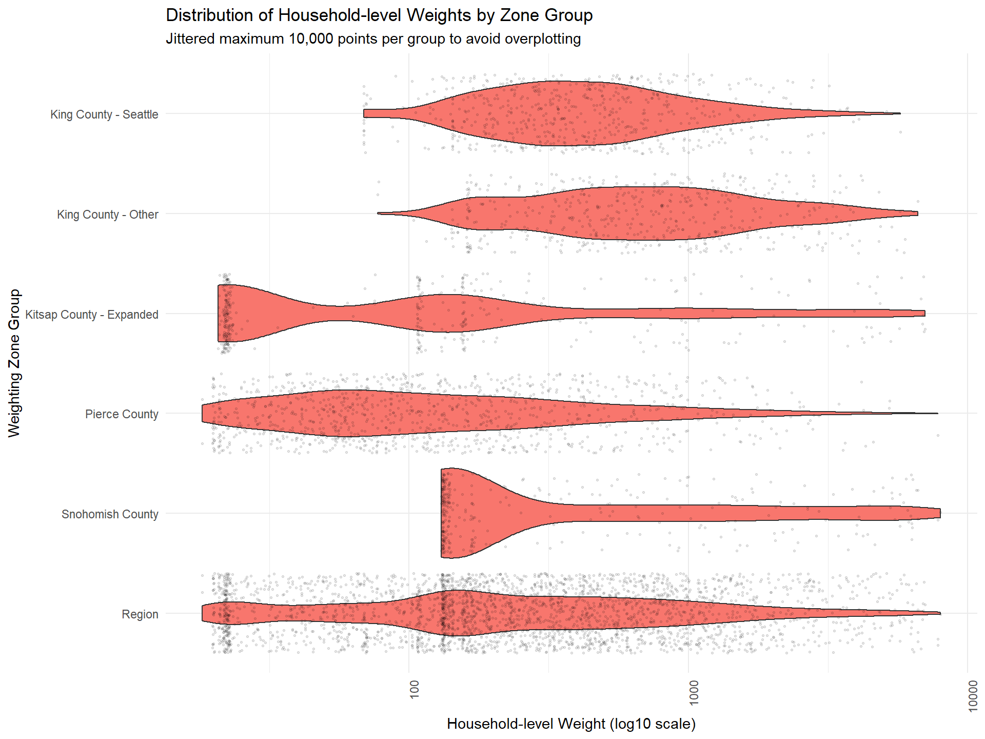
Figure: Fit error (MAPE) Variance (CV) and Multimodality (DIP statistic) of Weights by Maximum Expansion Factor and Maximum Weight Cap
This diagnostic figure summarizes how fit error (MAPE), weight variance (CV), and multimodality (Dip Statistic) change as weighting parameters (maximum expansion factor, weight cap) are varied in PopulationSim. These metrics help balance the goals of matching ACS targets and maintaining stable, unimodal weight distributions.
- MAPE: Mean Absolute Percentage Error, measures discrepancy between weighted survey estimates and targets.
- CV: Coefficient of Variation, indicates weight variability.
- Dip Statistic: Measures the degree to which weights deviate from a single peak (unimodality).
Interpretation note
Select weighting parameters where MAPE stabilizes, CV remains moderate, and Dip Statistic indicates unimodal distributions.
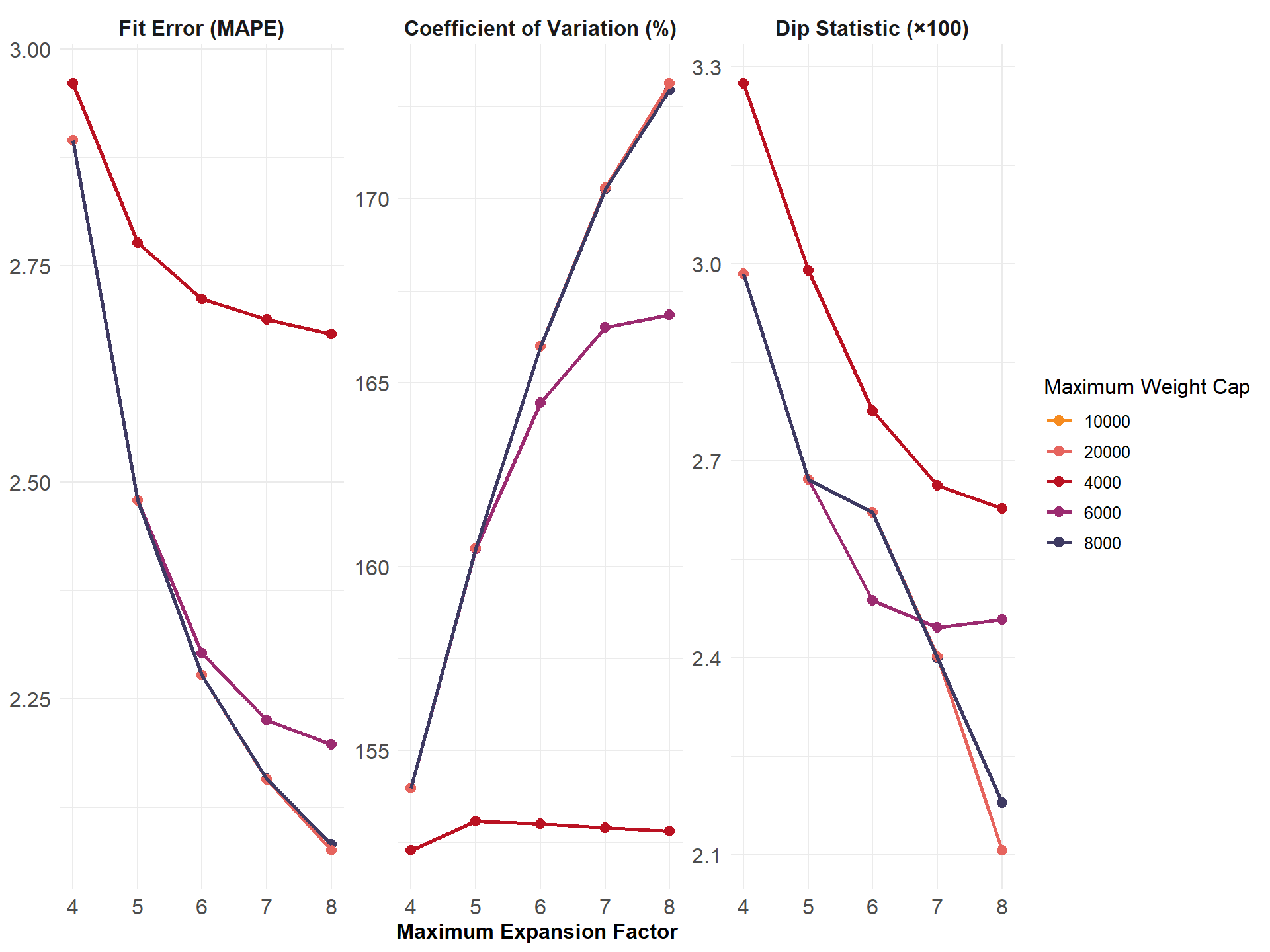
Table: Household- and Person-Level Weight Variability by Zone Group
The following table summarizes key variability statistics for the household- and person-level weights produced in Round 2. These statistics are calculated for each weighting zone group and for the region as a whole, using the maximum expansion factor applied in this weighting round.
- Household MAPE: Mean Absolute Percentage Error for household-level targets, indicating how closely weighted survey estimates match Census targets.
- Person MAPE: MAPE for person-level targets, showing fit to demographic controls.
- Coefficient of Variation: Standard deviation of weights divided by the mean, a normalized measure of weight variability.
Reviewing these metrics helps identify zones or groups where weights may be too variable or fit to targets may be weak.
Weighting zone group | N | Household MAPE | Person MAPE | Coefficient of variation |
|---|---|---|---|---|
King County - Seattle | 619 | 0.33 | 0.82 | 1.07 |
King County - Other | 518 | 0.29 | 0.39 | 1.03 |
Kitsap County - Expanded | 387 | 3.84 | 3.37 | 2.44 |
Pierce County | 1,050 | 0.23 | 0.42 | 2.02 |
Snohomish County | 336 | 1.81 | 1.35 | 1.74 |
Region | 2,910 | 0.75 | 0.86 | 1.70 |
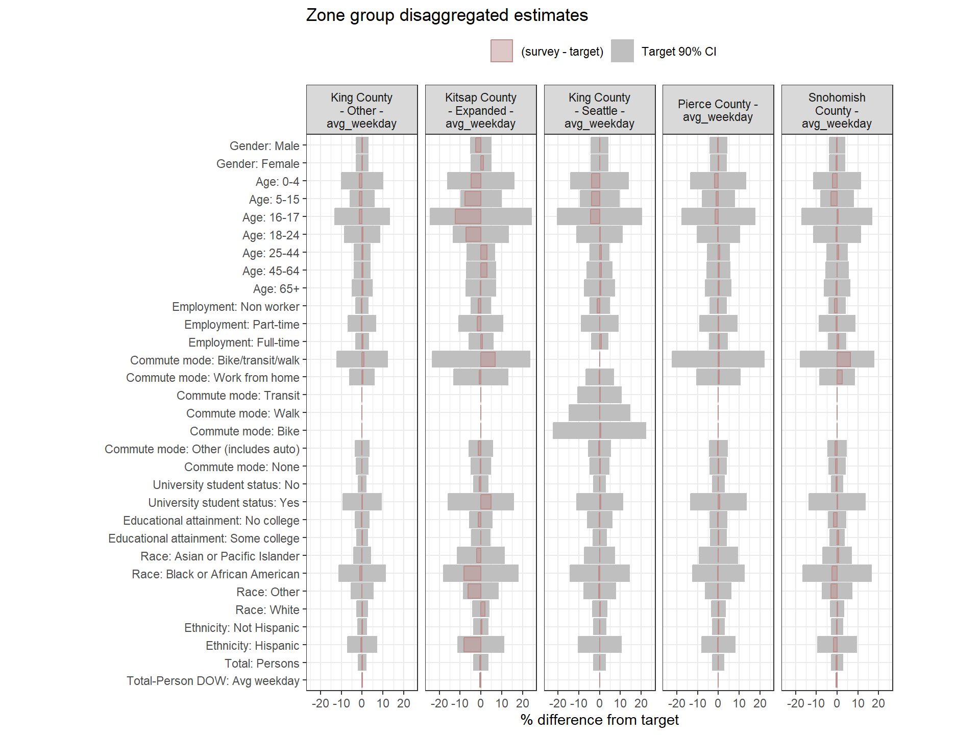
Round 2 Weight Fit to Targets
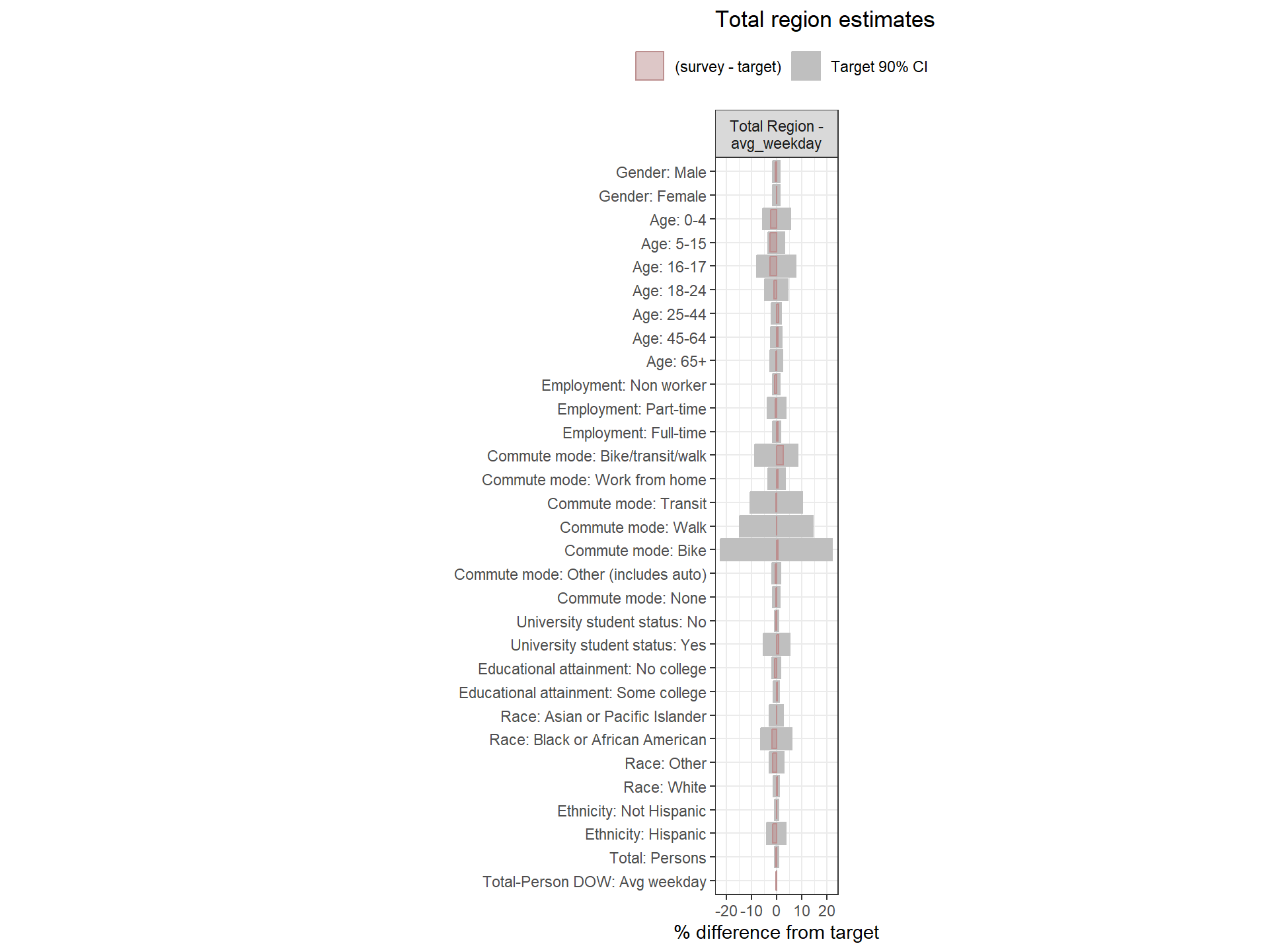
This section examines how well the weighted survey totals match the Census targets after Round 1 weighting. Each chart visualizes the percent difference between the weighted estimate and the target for each variable, alongside 90% confidence intervals around the target.
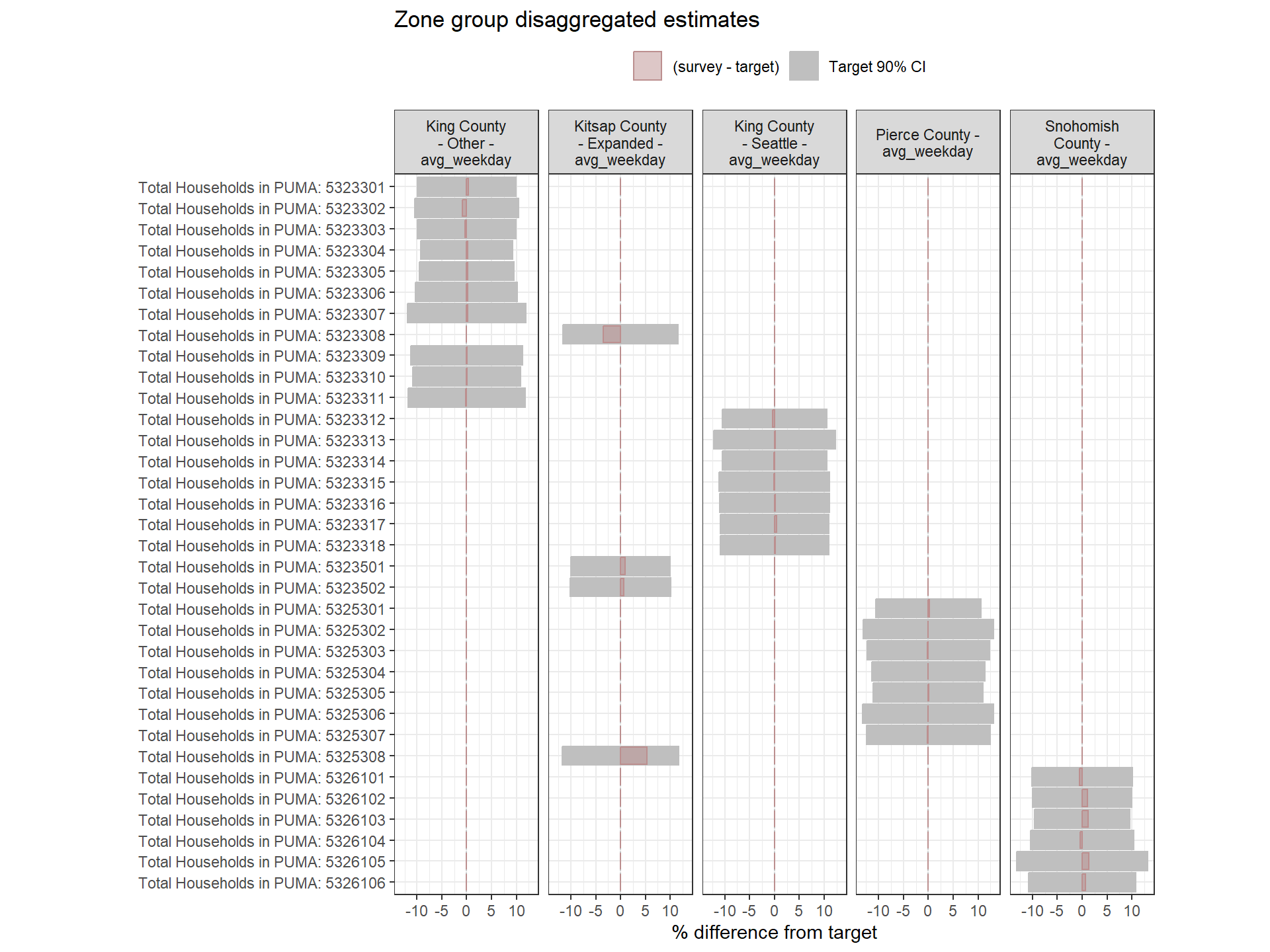
- Gray bars: 90% confidence interval as a percent of the target value.
- Red bars: Difference between the weighted survey estimate and the target. Negative bars indicate survey totals below the target.
If the red bar exceeds the confidence interval or if the interval itself is wide, this is a sign that the weighting approach may need adjustment. Red bars are bolded when error bounds are larger than desired (+/- 20% for regional estimates, +/- 25% for zone group estimates).
Weighting lever: Aggregate target categories
If some target categories or survey counts are very small, wide error margins may occur. Aggregating categories within certain zone groups or across the region can help minimize weight variance and produce more stable results. This should be considered after first adjusting weighting parameters.
Regional Weights Fit to Target Data
Figure: Household-Level Round 2 Weights Versus Target Estimates, by Day-of-Week
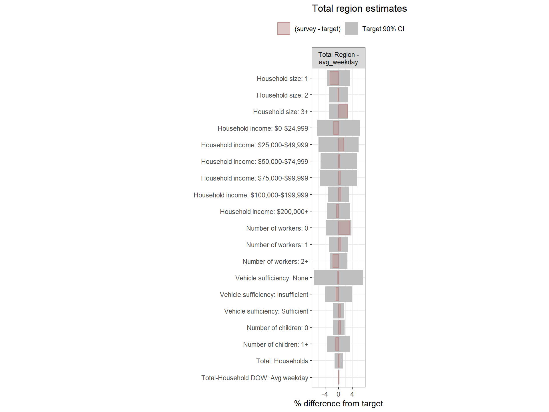
Figure: PUMA-Level Round 2 Weights Versus Target Estimates, by Day-of-Week
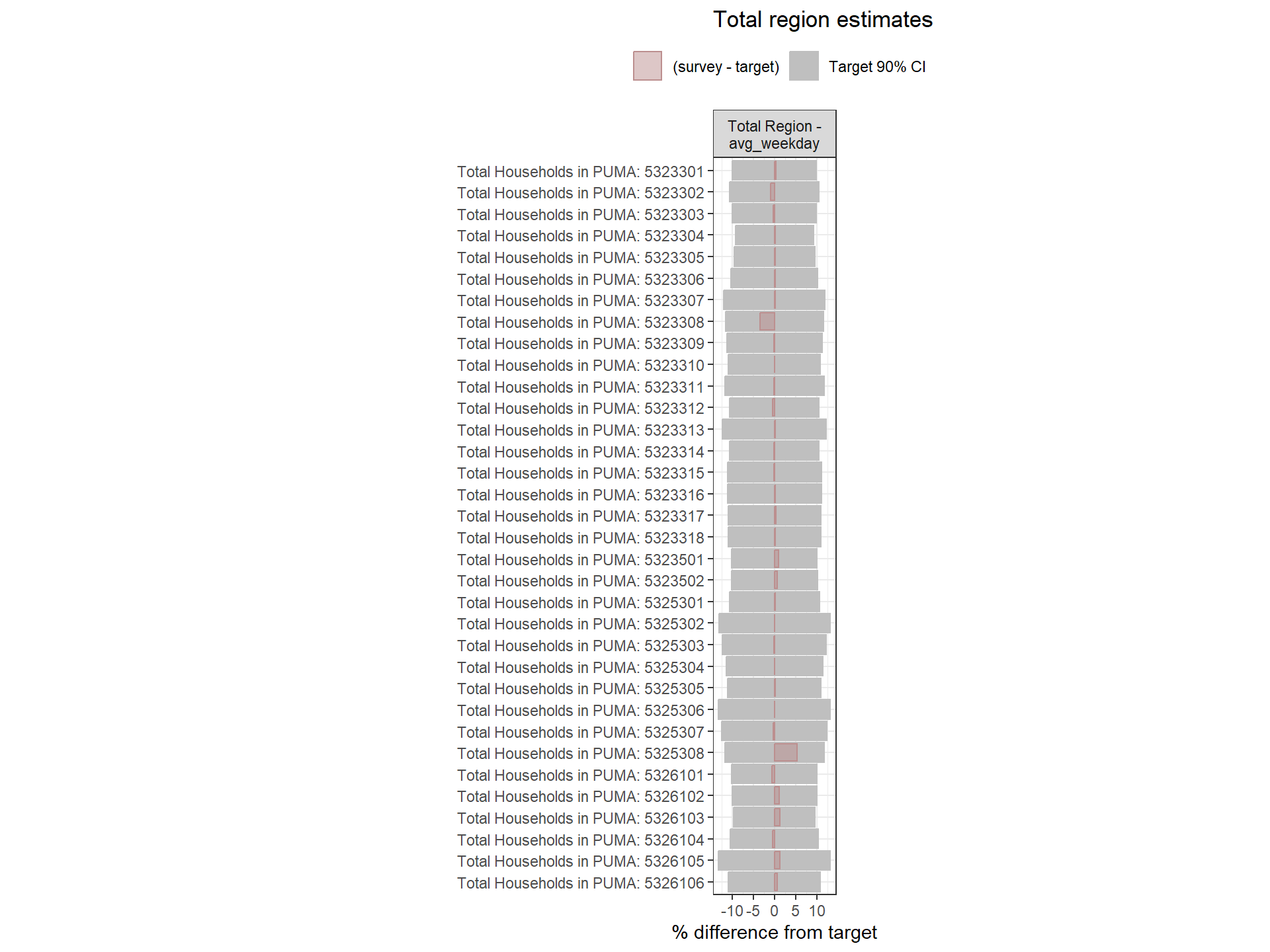
Figure: Person-Level Round 2 Weights Versus Target Estimates, by Day-of-Week
Weighting Zone Group Weights Fit to Target Data
Figure: Household-Level Round 2 Weights Versus Target Estimates, by Day-of-Week
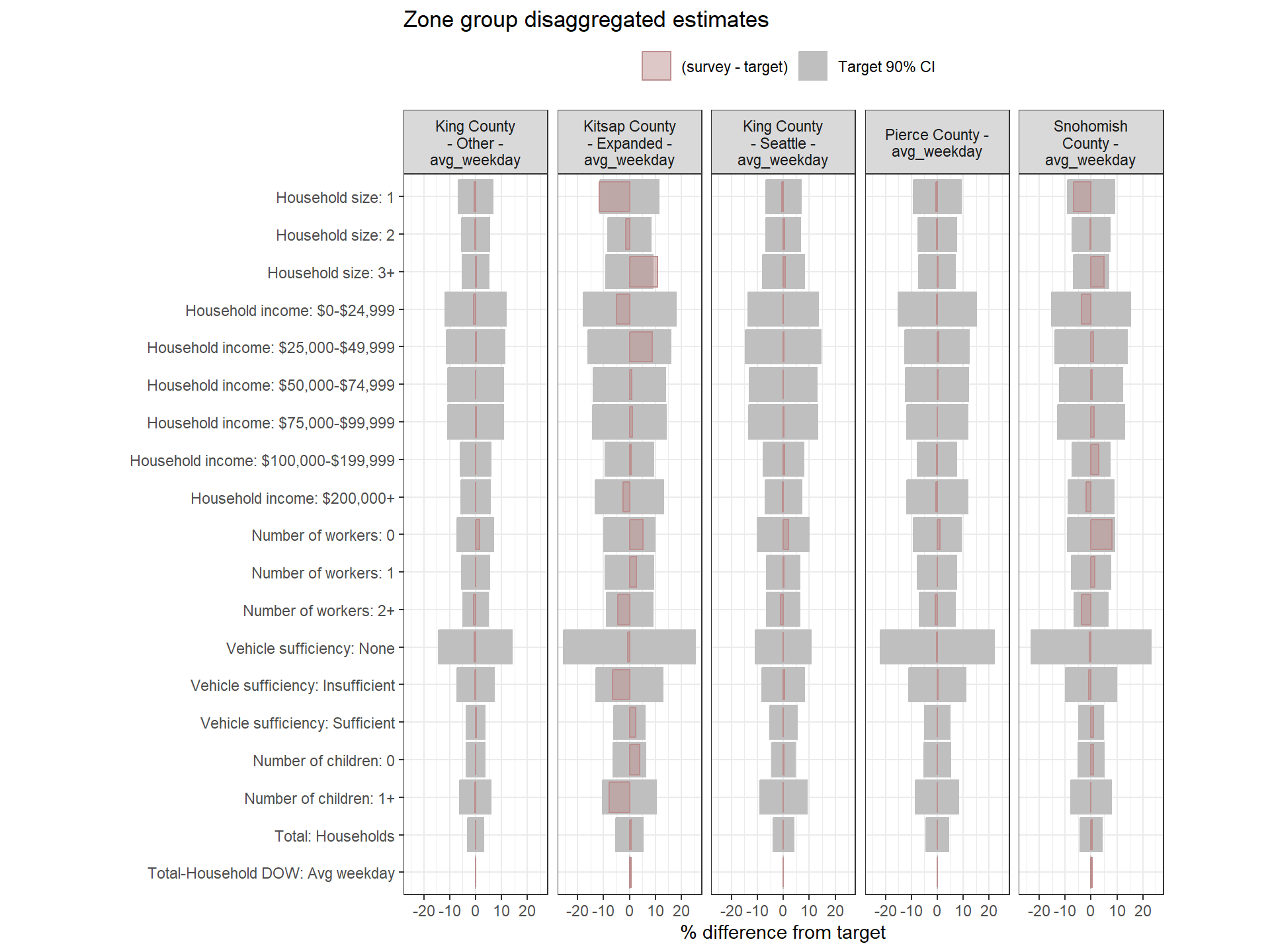
Figure: PUMA-Level Round 2 Weights Versus Target Estimates, by Day-of-Week
Person-Level Round 2 Weights Versus Target Estimates, by Day-of-Week